Part 3 Robust Bayesian statistics & applications in - PowerPoint PPT Presentation
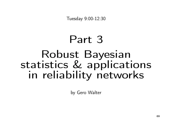
Tuesday 9:00-12:30 Part 3 Robust Bayesian statistics & applications in reliability networks by Gero Walter 69 Robust Bayesian statistics & applications in reliability networks Outline Robust Bayesian Analysis (9am) Why The
Tuesday 9:00-12:30 Part 3 Robust Bayesian statistics & applications in reliability networks by Gero Walter 69
Robust Bayesian statistics & applications in reliability networks Outline Robust Bayesian Analysis (9am) Why The Imprecise Dirichlet Model General Framework for Canonical Exponential Families Exercises I (9:30am) System Reliability Application (10am) Break (10:30am) Exercises II (11am) 70
Robust Bayesian statistics & applications in reliability networks Outline Robust Bayesian Analysis (9am) Why The Imprecise Dirichlet Model General Framework for Canonical Exponential Families Exercises I (9:30am) System Reliability Application (10am) Break (10:30am) Exercises II (11am) 71
Robust Bayesian Analysis: Why ◮ choice of prior can severely affect inferences even if your prior is ‘non-informative’ 72
Robust Bayesian Analysis: Why ◮ choice of prior can severely affect inferences even if your prior is ‘non-informative’ ◮ solution: systematic sensitivity analysis over prior parameters 72
Robust Bayesian Analysis: Why ◮ choice of prior can severely affect inferences even if your prior is ‘non-informative’ ◮ solution: systematic sensitivity analysis over prior parameters ◮ models from canonical exponential family make this easy to do [18] 72
Robust Bayesian Analysis: Why ◮ choice of prior can severely affect inferences even if your prior is ‘non-informative’ ◮ solution: systematic sensitivity analysis over prior parameters ◮ models from canonical exponential family make this easy to do [18] ◮ close relations to robust Bayes literature, e.g. [7, 19, 20] 72
Robust Bayesian Analysis: Why ◮ choice of prior can severely affect inferences even if your prior is ‘non-informative’ ◮ solution: systematic sensitivity analysis over prior parameters ◮ models from canonical exponential family make this easy to do [18] ◮ close relations to robust Bayes literature, e.g. [7, 19, 20] ◮ concerns uncertainty in the prior (uncertainty in data generating process: imprecise sampling models) 72
Robust Bayesian Analysis: Why ◮ choice of prior can severely affect inferences even if your prior is ‘non-informative’ ◮ solution: systematic sensitivity analysis over prior parameters ◮ models from canonical exponential family make this easy to do [18] ◮ close relations to robust Bayes literature, e.g. [7, 19, 20] ◮ concerns uncertainty in the prior (uncertainty in data generating process: imprecise sampling models) ◮ here: focus on imprecise Dirichlet model 72
Robust Bayesian Analysis: Why ◮ choice of prior can severely affect inferences even if your prior is ‘non-informative’ ◮ solution: systematic sensitivity analysis over prior parameters ◮ models from canonical exponential family make this easy to do [18] ◮ close relations to robust Bayes literature, e.g. [7, 19, 20] ◮ concerns uncertainty in the prior (uncertainty in data generating process: imprecise sampling models) ◮ here: focus on imprecise Dirichlet model ◮ if your prior is informative then prior-data conflict can be an issue [31, 29] (we’ll come back to this in the system reliability application) 72
Robust Bayesian Analysis: Principle of Indifference How to construct a prior if we do not have a lot of information? Laplace: Principle of Indifference Use the uniform distribution. Obvious issue: this depends on the parametrisation! 73
Robust Bayesian Analysis: Principle of Indifference How to construct a prior if we do not have a lot of information? Laplace: Principle of Indifference Use the uniform distribution. Obvious issue: this depends on the parametrisation! Example An object of 1kg has uncertain volume V between 1 ℓ and 2 ℓ . ◮ Uniform distribution over volume V = ⇒ E ( V ) = 1 . 5 ℓ . ◮ Uniform distribution over density ρ = 1 / V = ⇒ � 1 0 . 5 2 /ρ d ρ = 2 ( ln 1 − ln 0 . 5 ) = 1 . 39 ℓ E ( V ) = E ( 1 /ρ ) = 73
Robust Bayesian Analysis: Principle of Indifference How to construct a prior if we do not have a lot of information? Laplace: Principle of Indifference Use the uniform distribution. Obvious issue: this depends on the parametrisation! Example An object of 1kg has uncertain volume V between 1 ℓ and 2 ℓ . ◮ Uniform distribution over volume V = ⇒ E ( V ) = 1 . 5 ℓ . ◮ Uniform distribution over density ρ = 1 / V = ⇒ � 1 0 . 5 2 /ρ d ρ = 2 ( ln 1 − ln 0 . 5 ) = 1 . 39 ℓ E ( V ) = E ( 1 /ρ ) = The uniform distribution does not really model prior ignorance. (Jeffreys prior is transformation-invariant, but depends on the sample space and can break decision making!) 73
Robust Bayesian Analysis: Prior Ignorance via Sets of Probabilities How to construct prior if we do not have a lot of information? Boole: Probability Bounding Use the set of all probability distributions (vacuous model). Results no longer depend on parametrisation! 74
Robust Bayesian Analysis: Prior Ignorance via Sets of Probabilities How to construct prior if we do not have a lot of information? Boole: Probability Bounding Use the set of all probability distributions (vacuous model). Results no longer depend on parametrisation! Example An object of 1kg has uncertain volume V between 1 ℓ and 2 ℓ . ◮ Set of all distributions over volume V = ⇒ E ( V ) ∈ [ 1 , 2 ] . ◮ Set of all distribution over density ρ = 1 / V = ⇒ E ( V ) = E ( 1 /ρ ) ∈ [ 1 , 2 ] 74
Robust Bayesian Analysis: Prior Ignorance via Sets of Probabilities Theorem The set of posterior distributions resulting from a vacuous set of prior distributions is again vacuous, regardless of the likelihood. We can never learn anything when starting from a vacuous set of priors. 75
Robust Bayesian Analysis: Prior Ignorance via Sets of Probabilities Theorem The set of posterior distributions resulting from a vacuous set of prior distributions is again vacuous, regardless of the likelihood. We can never learn anything when starting from a vacuous set of priors. Solution: Near-Vacuous Sets of Priors Only insist that the prior predictive, or other classes of inferences, are vacuous. This can be done using sets of conjugate priors [4, 5]. 75
Robust Bayesian statistics & applications in reliability networks Outline Robust Bayesian Analysis (9am) Why The Imprecise Dirichlet Model General Framework for Canonical Exponential Families Exercises I (9:30am) System Reliability Application (10am) Break (10:30am) Exercises II (11am) 76
The Imprecise Dirichlet Model: Definition ◮ introduced by Peter Walley [27, 28] ◮ for multinomial sampling, k categories 1, 2, . . . , k ◮ Bayesian conjugate analysis ◮ multinomial likelihood (sample n = ( n 1 , . . . , n k ) , � n i = n ) k n ! � θ n i f ( n | θ ) = i n 1 ! · · · n k ! i = 1 ◮ conjugate Dirichlet prior ◮ with mean t = ( t 1 , . . . , t k ) = prior expected proportions ◮ and parameter s > 0 k Γ( s ) � θ st i − 1 f ( θ ) = i � k i = 1 Γ( st i ) i = 1 77
The Imprecise Dirichlet Model: Definition ◮ introduced by Peter Walley [27, 28] ◮ for multinomial sampling, k categories 1, 2, . . . , k ◮ Bayesian conjugate analysis ◮ multinomial likelihood (sample n = ( n 1 , . . . , n k ) , � n i = n ) k n ! � θ n i f ( n | θ ) = i n 1 ! · · · n k ! i = 1 ◮ conjugate Dirichlet prior ◮ with mean t = ( t 1 , . . . , t k ) = prior expected proportions ◮ and parameter s > 0 k Γ( s ) � θ st i − 1 f ( θ ) = i � k i = 1 Γ( st i ) i = 1 Definition (Imprecise Dirichlet Model) Use the set M ( 0 ) of all Dirichlet priors, for a fixed s > 0, and take the infimum/supremum over t of the posterior to get lower/upper predictive probabilities/expectations. 77
The Imprecise Dirichlet Model: Properties ◮ conjugacy: f ( θ | n ) again Dirichlet with parameters i = st i + n i s n n i t ∗ = s + n t i + n , s + n s + n s ∗ = s + n ◮ t ∗ i = E ( θ i | n ) = P ( i | n ) is a weighted average of t i and n i / n , with weights proportional to s and n , respectively ◮ s can be interpreted as a prior strength or pseudocount ◮ lower and upper expectations / probabilities by min and max over t ∈ ∆ (unit simplex) 78
The Imprecise Dirichlet Model: Properties Posterior predictive probabilities ◮ for observing a particular category n i P ( i | n ) = s + n i P ( i | n ) = s + n , s + n ◮ for observing a non-trivial event A ⊆ { 1 , . . . , k } P ( A | n ) = s + n A n A P ( A | n ) = s + n , s + n , with n A = � i ∈ A n i Satisfies prior near ignorance: vacuous for prior predictive P ( A ) = 0 , P ( A ) = 1 Inferences are independent of categorisation (‘Representation Invariance Principle’). 79
The Imprecise Dirichlet Model: Why A Set of Priors? ◮ single prior = ⇒ dependence on categorisation ◮ for example, single Dirichlet prior (with t A = � i ∈ A t i , s = 2) P ( A | n ) = 2 t A + n A n + 2 one red marble observed ◮ two categories red (R) and other (O): ⇒ t R = t O = 1 ⇒ P ( R | n ) = 2 prior ignorance = 2 = 3 ◮ three categories red (R), green (G), and blue (B): ⇒ t R = t G = t B = 1 ⇒ P ( R | n ) = 5 prior ignorance = 3 = 9 80
Recommend
More recommend
Explore More Topics
Stay informed with curated content and fresh updates.










![Bayesian Networks [KF] Chapter 3 University of Waterloo CS 786 Lecture 2: May 3rd, 2012](https://c.sambuz.com/996390/bayesian-networks-kf-chapter-3-s.webp)
