ParameterEstimation October 22, 2018 1 Lecture 18: Parameter - PDF document
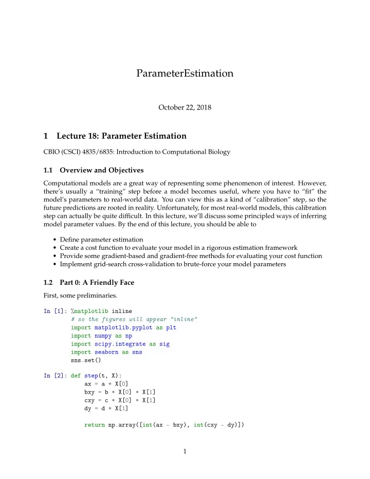
ParameterEstimation October 22, 2018 1 Lecture 18: Parameter Estimation CBIO (CSCI) 4835/6835: Introduction to Computational Biology 1.1 Overview and Objectives Computational models are a great way of representing some phenomenon of interest.
ParameterEstimation October 22, 2018 1 Lecture 18: Parameter Estimation CBIO (CSCI) 4835/6835: Introduction to Computational Biology 1.1 Overview and Objectives Computational models are a great way of representing some phenomenon of interest. However, there’s usually a “training” step before a model becomes useful, where you have to “fit” the model’s parameters to real-world data. You can view this as a kind of “calibration” step, so the future predictions are rooted in reality. Unfortunately, for most real-world models, this calibration step can actually be quite difficult. In this lecture, we’ll discuss some principled ways of inferring model parameter values. By the end of this lecture, you should be able to • Define parameter estimation • Create a cost function to evaluate your model in a rigorous estimation framework • Provide some gradient-based and gradient-free methods for evaluating your cost function • Implement grid-search cross-validation to brute-force your model parameters 1.2 Part 0: A Friendly Face First, some preliminaries. In [1]: %matplotlib inline # so the figures will appear "inline" import matplotlib.pyplot as plt import numpy as np import scipy.integrate as sig import seaborn as sns sns.set() In [2]: def step(t, X): ax = a * X[0] bxy = b * X[0] * X[1] cxy = c * X[0] * X[1] dy = d * X[1] return np.array([int(ax - bxy), int(cxy - dy)]) 1
Anyone recognize this differential equation? Predator-Prey equations! (aka, the Lotka-Volterra model for competition) What do you think about this line? return np.array([int(ax - bxy), int(cxy - dy)]) A slight tweak from Lecture 15–the addition of the int() castings on both populations! What effect will this have? Populations can now go to 0! And if one does go to zero, it never recovers. In [3]: def plot_pp(x, y, labels): """ This function just plots the data, given the x and y axes, and the labels for each. """ plt.plot(x, y[0], label = labels[0]) plt.plot(x, y[1], label = labels[1]) plt.ylim([0, y.max() + 2]) # Fix the bottom of the y-axis at 0 so we can always see plt.legend(loc = 0) In [4]: # These are all taken straight out of Lecture 15. a = 1.0 # Prey growth b = 0.1 # Predation rate c = 0.075 # Predator growth d = 1.0 # Predator death In [5]: t = [0, 15] dt = np.linspace(t[0], t[1], 10000) X0 = np.array([10, 5]) X = sig.solve_ivp(step, t, X0, t_eval = dt) print(X["message"]) print("Success?", X["success"]) The solver successfully reached the end of the integration interval. Success? True In [6]: labels = ["Prey", "Predator"] plot_pp(X["t"], X["y"], labels) 2
In [7]: X0 = np.array([100, 5]) X = sig.solve_ivp(step, t, X0, t_eval = dt) plot_pp(X["t"], X["y"], labels) 3
In [8]: X0 = np.array([100, 1]) X = sig.solve_ivp(step, t, X0, t_eval = dt) plot_pp(X["t"], X["y"], labels) In [9]: X0 = np.array([10, 10]) X = sig.solve_ivp(step, t, X0, t_eval = dt) plot_pp(X["t"], X["y"], labels) 4
In [10]: X0 = np.array([10, 100]) X = sig.solve_ivp(step, t, X0, t_eval = dt) plot_pp(X["t"], X["y"], labels) 5
gaussianscatterplot This seems like a lot of work to figure out what combinations of initial population values result in one or both species going extinct.. . The main question of this lecture: Is there a better way? The main point of this lecture: Yes, and here’s how! 1.3 Part 1: What is “parameter estimation”? Recall what a model is: • A “summary” of our understanding of a system (e.g., a biological mechanism) • Enables predictions that test our own understanding • Describes aspects of a system that may not be directly accessible via observation To function, almost every model ever has some associated “numbers”, so-called parameters . (remember Gaussian/Normal/bell-curve distributions? they have two parameters: a mean , and a variance ) Even if a model is “almost correct”, their parameters usually need some “reasonable” numeri- cal values to function properly. How do we choose these parameters? If I had the following scatter plot of data and wanted to “fit” a 2D Gaussian model to it, what would I choose for the mean and (co)variance? 6
expdata expdata A mean of (0, 0) and a covariance around +/- 100 would be a decent guess. If you have a case like the last one where it’s one small set of data that you can visualize (e.g., in 2D or 3D), just a handful of parameters you need to set (e.g., a mean and a covariance), and you can easily verify “correctness”, then absolutely go for it! Alternatively, the literature can often have experimentally-determined values (i.e., other re- searchers that have already done what I just described) that you can plug in and verify yourself. **Unfortunately. . . * • Data are frequently much higher-dimensional than just 2D or 3D (i.e., they’re really hard to visualize as a way of “checking” your parameter values–how about a 10D Gaussian?) • Data are getting bigger . If it took you a few hours to calculate a single model from your data, you’d have a hard time doing “guess-and-check” with each one in a reasonable amount of time. • Visual “guess-and-check” for validation of model parameters isn’t always a feasiable strat- egy. Even with our toy Lotka-Volterra model, it would be really hard to figure out a decent definition of “best” parameter values in a reasonable amount of time. We need a more automated, computational approach to inferring parameters from experi- mental data. 1.3.1 The setup: experimental data First, you have your experimental data that you want to model. 1.3.2 The setup: model Next, you have your model that you want to “fit”. 7
expdata expdata 1.3.3 The setup: cost function Third, and most importantly, you have a cost function . What is a “cost function”? Formally, it’s an equation that quantifies the discrepancy between your experimental data and your model’s predictions. Informally, it’s a precise way of “nudging” your model’s parameters in a direction that makes the predictions of your model more closely resemble reality. As such, creating an effective cost function is critical –a bad cost function will result in a bad model. There are several ways of developing and solving cost functions to set your model parame- ters. We’ll discuss a few here. 1.4 Part 2: Gradient-based methods Remember how we said a cost function is critical to evaluating your model? That’s because a well-defined cost function–indeed, like any other function–can have a derivative (or gradient , in high dimensions). The “cost” function is so-named to provide us with some intuition about how we need to use it to find the “best” parameters for our model. • When the cost function has a high value, this means there is a high cost to using the cor- responding model parameters. Intuitively, this usually means the model parameters don’t reflect reality very well. 8
• Conversely, when the cost function has a low value, this means there is a low cost to using the corresponding model parameters. Usually, this means the model parameters have a good alignment with the real-world. So if the goal is to make the cost function have a low value–does anyone remember how to find the minimum of a function f ( x ) ? Take the derivative, set it equal to zero, and solve! 1.4.1 That’s it, you’re done! . . . unfortunately, not quite. Let’s illustrate by creating a cost function for our Lotka-Volterra model. A cost function is an excellent opportunity to encode your domain knowledge into the prob- lem. What, in your mind, would constitute a “good” Lotka-Volterra model of stabile predator- prey populations? Here’s my list: - Neither population goes to 0 (no one goes extinct) - Of the non-extinct popu- lations, I like the ones where the two find as stable an equilibrium as possible (the absolute values of the populations change as little as possible) How could we design a “cost” function to encourage this behavior? (in terms of “high” and “low” costs) • Impose a “high” cost whenever one or both populations go to 0 • Impose a cost that is inversely proportional to how much the two populations vary 1.4.2 My cost function In [11]: def my_cost_func(Y): """ My little cost function, where Y is a tuple with the initial prey and predator populations. """ a = 1.0 b = 0.1 c = 0.075 d = 1.0 t = [0, 15] dt = np.linspace(t[0], t[1], 10000) X = sig.solve_ivp(step, t, Y, t_eval = dt) y_prey, y_pred = X["y"] # First: if either population went to 0, # we want to give it the maximum possible cost. if y_prey[-1] == 0 or y_pred[-1] == 0: # This is a little cheat that returns the # maximum possible float value NumPy can store # (note: it's a really, really big number) return np.finfo(np.float).max # If both populations were non-zero, let's create 9
Recommend
More recommend
Explore More Topics
Stay informed with curated content and fresh updates.
