Pair-comparison studies Extended Bradley-Terry models Sport : player - PDF document

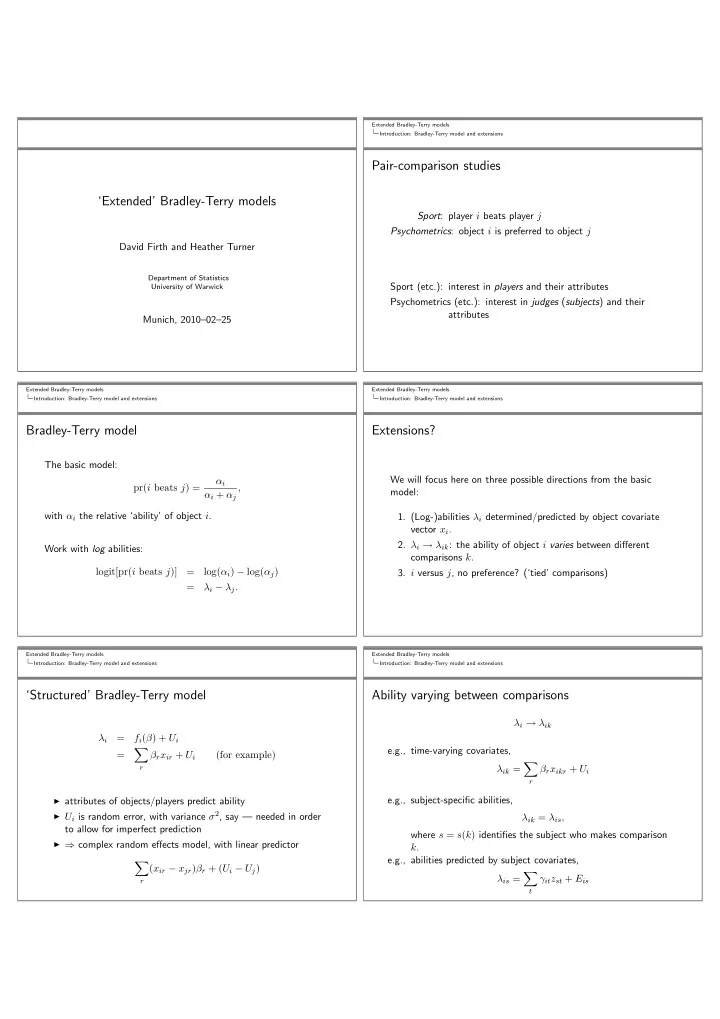
Extended Bradley-Terry models Introduction: Bradley-Terry model and extensions Pair-comparison studies ‘Extended’ Bradley-Terry models Sport : player i beats player j Psychometrics : object i is preferred to object j David Firth and Heather Turner Department of Statistics Sport (etc.): interest in players and their attributes University of Warwick Psychometrics (etc.): interest in judges ( subjects ) and their attributes Munich, 2010–02–25 Extended Bradley-Terry models Extended Bradley-Terry models Introduction: Bradley-Terry model and extensions Introduction: Bradley-Terry model and extensions Bradley-Terry model Extensions? The basic model: We will focus here on three possible directions from the basic α i pr( i beats j ) = , model: α i + α j with α i the relative ‘ability’ of object i . 1. (Log-)abilities λ i determined/predicted by object covariate vector x i . 2. λ i → λ ik : the ability of object i varies between different Work with log abilities: comparisons k . logit[pr( i beats j )] = log( α i ) − log( α j ) 3. i versus j , no preference? (‘tied’ comparisons) = λ i − λ j . Extended Bradley-Terry models Extended Bradley-Terry models Introduction: Bradley-Terry model and extensions Introduction: Bradley-Terry model and extensions ‘Structured’ Bradley-Terry model Ability varying between comparisons λ i → λ ik λ i = f i ( β ) + U i e.g., time-varying covariates, � = β r x ir + U i (for example) � r λ ik = β r x ikr + U i r ◮ attributes of objects/players predict ability e.g., subject-specific abilities, ◮ U i is random error, with variance σ 2 , say — needed in order λ ik = λ is , to allow for imperfect prediction where s = s ( k ) identifies the subject who makes comparison ◮ ⇒ complex random effects model, with linear predictor k . e.g., abilities predicted by subject covariates, � ( x ir − x jr ) β r + ( U i − U j ) � λ is = γ it z st + E is r t

Extended Bradley-Terry models Extended Bradley-Terry models Introduction: Bradley-Terry model and extensions Introduction: Bradley-Terry model and extensions Ability varying between comparisons (continued) Ties What to do when neither i nor j is preferred? e.g., still with abilities λ is varying between subjects, a particular Elaborate the Bradley-Terry model? (Rao and Kupper, 1967; form likely to be useful is multiplicative interaction, Davidson, 1970) �� � λ is = λ i exp γ t z st + E is t A crude alternative approach/approximation: tie = half a ‘win’ for each of i and j This last form is not yet implemented in the BradleyTerry2 package; it will require features from the gnm (generalized nonlinear models) package. Suggests a generalization: half → some other fraction? Extended Bradley-Terry models Extended Bradley-Terry models Implementation in R: The BradleyTerry2 package Implementation in R: The BradleyTerry2 package Implementation in R : The BradleyTerry2 package CEMS Data Main new features The CEMS data (Dittrich et al, 1998) concern the preferences of ◮ flexible formula interface to modelling fitting function BTm() : students in selecting a school from the Community of European allows object-specific, subject-specific, contest-specific Management Schools for their international visit. variables and random effects [limited implementation] ◮ efficient data management of multiple data frames ◮ 6 CEMS schools are covered in the survey ◮ students were to choose between each pair of schools (ties Best of original BradleyTerry package allowed) ◮ further data collected on students e.g. type of degree, ◮ translation of formula to appropriate design matrix language skills ◮ methods for fitted model object, e.g. anova, BTabilities ◮ missing data handling Extended Bradley-Terry models Extended Bradley-Terry models Implementation in R: The BradleyTerry2 package Implementation in R: The BradleyTerry2 package Data Structure Model Specification > library(BradleyTerry2); data(CEMS); str(CEMS) List of 3 Model specifiation is controlled by four arguments to BTm() $ preferences:’data.frame’: 4545 obs. of 8 variables: ..$ student : num [1:4545] 1 1 1 1 1 1 1 1 1 1 ... outcome a binomial response as accepted by glm() . ..$ school1 : Factor w/ 6 levels "Barcelona","London",..: 2 2 4 ..$ school2 : Factor w/ 6 levels "Barcelona","London",..: 4 3 3 player1, player2 specify the players in each contest and any ..$ win1 : num [1:4545] 1 1 NA 0 0 0 1 1 0 1 ... other player-specific contest variables in data frames ... with the same attributes. $ students :’data.frame’: 303 obs. of 8 variables: ..$ STUD: Factor w/ 2 levels "other","commerce": 1 2 1 2 1 1 1 2 id the name of the factor in player1/player2 that ..$ ENG : Factor w/ 2 levels "good","poor": 1 1 1 1 2 1 1 1 2 1 gives the identity of the player. ... formula a one-sided formula for player ability. $ schools :’data.frame’: 6 obs. of 7 variables: ..$ Barcelona: num [1:6] 1 0 0 0 0 0 ..$ London : num [1:6] 0 1 0 0 0 0 ...

Extended Bradley-Terry models Extended Bradley-Terry models Implementation in R: The BradleyTerry2 package Implementation in R: The BradleyTerry2 package Standard Bradley Terry Model Model Summaries For models with no random effects, BTm returns an object which is essentially a "glm" object, hence the usual model summaries can A Bradley-Terry model with a separate ability for each player can be obtained, e.g. print() : be specified as follows Bradley Terry model fit by glm.fit > standardBT <- BTm(outcome = cbind(win1.adj, win2.adj), player1 = data.frame(school = school1), Call: BTm(outcome = cbind(win1.adj, win2.adj), player1 = school1, player2 = data.frame(school = school2), player2 = school2, formula = ~.., refcat = "Stockholm", id = "school", formula = ~ school, data = CEMS$preferences) refcat = "Stockholm", Coefficients: data = CEMS$preferences) ..Barcelona ..London ..Milano ..Paris ..St.Gallen Or we can use the default id , ".." 0.5379 1.5975 0.3878 0.9064 0.5251 > standardBT <- BTm(outcome = cbind(win1.adj, win2.adj), Degrees of Freedom: 4454 Total (i.e. Null); 4449 Residual (91 observations deleted due to missingness) player1 = school1, player2 = school2, Null Deviance: 5499 formula = ~ .., refcat = "Stockholm", Residual Deviance: 4929 AIC: 5854 data = CEMS$preferences) Warning message: In eval(expr, envir, enclos) : non-integer counts in a binomial glm! Extended Bradley-Terry models Extended Bradley-Terry models Implementation in R: The BradleyTerry2 package Implementation in R: The BradleyTerry2 package Object and Subject Variables Interaction Model > summary(interactionBT)$coef[, 1:2]/1.75 The final model in Dittrich et al, incorporating interactions with Estimate Std. Error subject-covariates, can be estimated as follows ..Barcelona 1.0363917 0.10184195 ..London 1.2734839 0.10523535 > interactionBT <- BTm(outcome = cbind(win1.adj, win2.adj), ..Milano 1.1136211 0.10030192 player1 = school1, player2 = school2, ..Paris 0.6453467 0.05797807 formula = ~ .. + ..St.Gallen 0.2487781 0.05663021 WOR[student]yes:LAT[..] 0.5933091 0.12278686 WOR[student] * LAT[..] + DEG[student]yes:St.Gallen[..] 0.2726479 0.06875424 DEG[student] * St.Gallen[..] + STUD[student]commerce:Paris[..] 0.4073965 0.07352900 STUD[student] * (Paris[..] + St.Gallen[..]) + St.Gallen[..]:STUD[student]commerce -0.1984449 0.07089058 ENG[student] * St.Gallen[..] + St.Gallen[..]:ENG[student]poor 0.1449582 0.07241576 FRA[student] * (London[..] + Paris[..]) + FRA[student]poor:London[..] -0.1607138 0.07519284 SPA[student] * Barcelona[..] + Paris[..]:FRA[student]poor -0.7142351 0.07132559 SPA[student]poor:Barcelona[..] -0.8409595 0.10336192 ITA[student] * (London[..] + Milano[..]) + London[..]:ITA[student]poor -0.2967857 0.10342156 SEX[student] * Milano[..], ITA[student]poor:Milano[..] -0.9603892 0.10386091 refcat = "Stockholm", data = CEMS) Milano[..]:SEX[student]male -0.1743107 0.06848606 Extended Bradley-Terry models Extended Bradley-Terry models Implementation in R: The BradleyTerry2 package Implementation in R: The BradleyTerry2 package Baseball Data Standard Bradley-Terry Model > (baseballModel1 <- BTm(cbind(home.wins, away.wins), home.team, away.team, data = baseball, id = "team")) Bradley Terry model fit by glm.fit The baseball data (Agresti, 2002) gives the results for 7 teams of the Eastern Division of the American League during the 1987 Call: BTm(outcome = cbind(home.wins, away.wins), season: player1 = home.team, player2 = away.team, id = "team", > str(baseball) data = baseball) ’data.frame’: 42 obs. of 4 variables: Coefficients: $ home.team: Factor w/ 7 levels "Baltimore","Boston",..: 5 5 5 5 5 teamBoston teamCleveland teamDetroit teamMilwaukee $ away.team: Factor w/ 7 levels "Baltimore","Boston",..: 4 7 6 2 3 1.1077 0.6839 1.4364 1.5814 $ home.wins: int 4 4 4 6 4 6 3 4 4 6 ... teamNew York teamToronto $ away.wins: int 3 2 3 1 2 0 3 2 3 0 ... 1.2476 1.2945 Degrees of Freedom: 42 Total (i.e. Null); 36 Residual Null Deviance: 78.02 Residual Deviance: 44.05 AIC: 140.5