P4 - Central Limit Theorem STAT 587 (Engineering) Iowa State - PowerPoint PPT Presentation
P4 - Central Limit Theorem STAT 587 (Engineering) Iowa State University August 28, 2020 Main Idea: Sums and averages of iid random variables from any distribution have approximate normal distributions for sufficiently large sample sizes.
P4 - Central Limit Theorem STAT 587 (Engineering) Iowa State University August 28, 2020 Main Idea: Sums and averages of iid random variables from any distribution have approximate normal distributions for sufficiently large sample sizes.
Bell-shaped curve Bell-shaped curve The term bell-shaped curve typically refers to the probability density function for a normal random variable: Bell−shaped curve Probability density function Value
Bell-shaped curve Histograms of samples from bell-shaped curves Histograms of 1,000 standard normal random variables 1 2 Number 3 4 Value
Bell-shaped curve Yield https://journals.plos.org/plosone/article?id=10.1371/journal.pone.0184198
Bell-shaped curve Examples SAT scores https://blogs.sas.com/content/iml/2019/03/04/visualize-sat-scores-nc.html
Bell-shaped curve Examples Histograms of samples from bell-shaped curves Histograms of 20 standard normal random variables 1 2 Number 3 4 Value
Bell-shaped curve Examples Tensile strength https://www.researchgate.net/figure/Comparison-of-histograms-for-BTS-and-tensile-strength-estimated-from-point-load_fig5_260617256
Central Limit Theorem Sums and averages of iid random variables Suppose X 1 , X 2 , . . . are iid random variables with V ar [ X i ] = σ 2 . E [ X i ] = µ Define Sample Sum: S n = X 1 + X 2 + · · · + X n Sample Average: X n = S n /n. For S n , we know SD [ S n ] = √ nσ. V ar [ S n ] = nσ 2 , E [ S n ] = nµ, and For X n , we know SD [ X n ] = σ/ √ n. V ar [ X n ] = σ 2 /n, E [ X n ] = µ, and
Central Limit Theorem Central Limit Theorem (CLT) Suppose X 1 , X 2 , . . . are iid random variables with V ar [ X i ] = σ 2 . E [ X i ] = µ Define Sample Sum: S n = X 1 + X 2 + · · · + X n Sample Average: X n = S n /n. Then the Central Limit Theorem says X n − µ S n − nµ d d lim → N (0 , 1) and lim → N (0 , 1) . σ/ √ n √ nσ n →∞ n →∞ Main Idea: Sums and averages of iid random variables from any distribution have approximate normal distributions for sufficiently large sample sizes.
Central Limit Theorem Yield https://journals.plos.org/plosone/article?id=10.1371/journal.pone.0184198
Central Limit Theorem Approximating distributions Approximating distributions Rather than considering the limit, I typically think of the following approximations as n gets large. For the sample average, · ∼ N ( µ, σ 2 /n ) . X n · where ∼ indicates approximately distributed because � � � � = σ 2 /n. E X n = µ and V ar X n For the sample sum, · ∼ N ( nµ, nσ 2 ) S n because E [ S n ] = nµ V ar [ S n ] = nσ 2 .
Central Limit Theorem Normal approximations to uniform Averages and sums of uniforms ind Let X i ∼ Unif (0 , 1) . Then µ = E [ X i ] = 1 σ 2 = V ar [ X i ] = 1 and 12 . 2 Thus � 1 1 � · X n ∼ N 2 , 12 n and � n 2 , n � · S n ∼ N . 12
Central Limit Theorem Normal approximations to uniform Averages of uniforms Histogram of d$mean 40 30 Density 20 10 0 0.47 0.48 0.49 0.50 0.51 0.52 0.53 0.54 d$mean
Central Limit Theorem Normal approximations to uniform Sums of uniforms Histogram of d$sum 0.04 Density 0.02 0.00 470 480 490 500 510 520 530 540 d$sum
Central Limit Theorem Normal approximation to a binomial Normal approximation to a binomial ind Recall if Y n = � n i =1 X i where X i ∼ Ber ( p ) , then Y n ∼ Bin ( n, p ) . For a binomial random variable, we have E [ Y n ] = np and V ar [ Y n ] = np (1 − p ) . By the CLT, Y n − np lim → N (0 , 1) , � n →∞ np (1 − p ) if n is large, · Y n ∼ N ( np, np [1 − p ]) .
Central Limit Theorem Roulette example Roulette example A European roulette wheel has 39 slots: one green, 19 black, and 19 red. If I play black every time, what is the probability that I will have won more than I lost after 99 spins of the wheel? https://isorepublic.com/photo/roulette-wheel/
Central Limit Theorem Roulette example Roulette example A European roulette wheel has 39 slots: one green, 19 black, and 19 red. If I play black every time, what is the probability that I will have won more than I lost after 99 spins of the wheel? Let Y indicate the total number of wins and assume Y ∼ Bin ( n, p ) with n = 99 and p = 19 / 39 . The desired probability is P ( Y ≥ 50) . Then P ( Y ≥ 50) = 1 − P ( Y < 50) = 1 − P ( Y ≤ 49) n = 99 p = 19/39 1-pbinom(49, n, p) [1] 0.399048
Central Limit Theorem Roulette example Roulette example A European roulette wheel has 39 slots: one green, 19 black, and 19 red. If I play black every time, what is the probability that I will have won more than I lost after 99 spins of the wheel? Let Y indicate the total number of wins. We can approximate Y using X ∼ N ( np, np (1 − p )) . P ( Y ≥ 50) ≈ 1 − P ( X < 50) 1-pnorm(50, n*p, sqrt(n*p*(1-p))) [1] 0.3610155 A better approximation can be found using a continuity correction.
Central Limit Theorem Astronomy example Astronomy example An astronomer wants to measure the distance, d , from Earth to a star. Suppose the procedure has a known standard deviation of 2 parsecs. The astronomer takes 30 iid measurements and finds the average of these measurements to be 29.4 parsecs. What is the probability the average is within 0.5 parsecs? http://planetary-science.org/astronomy/distance-and-magnitudes/
Central Limit Theorem Astronomy example Astronomy example Let X i be the i th measurement. The astronomer assumes that X 1 , X 2 , . . . X n are iid with E [ X i ] = d and V ar [ X i ] = σ 2 = 2 2 . The estimate of d is X n = ( X 1 + X 2 + · · · + X n ) = 29 . 4 . n ∼ N ( d, σ 2 /n ) · and, by the Central Limit Theorem, X n where n = 30 . We want to find � � � � P | X n − d | < 0 . 5 = P − 0 . 5 < X n − d < 0 . 5 � � − 0 . 5 30 < X n − d 0 . 5 = P σ/ √ n < √ √ 2 / 2 / 30 ≈ P ( − 1 . 37 < Z < 1 . 37) diff(pnorm(c(-1.37,1.37))) [1] 0.8293131
Central Limit Theorem Astronomy example Astronomy example - sample size Suppose the astronomer wants to be within 0.5 parsecs with at least 95% probability. How many more samples would she need to take? We solve � < . 5 �� � � � � 0 . 95 ≤ P � X n − d = P − 0 . 5 < X n − d < 0 . 5 � � 2 / √ n < X n − d − 0 . 5 0 . 5 = P σ/ √ n < 2 / √ n z = 0 . 5 / (2 / √ n ) = P ( − z < Z < z ) = 1 − [ P ( Z < − z ) + P ( Z > z )] = 1 − 2 P ( Z < − z ) where z = 1 . 96 since 1-2*pnorm(-1.96) [1] 0.9500042 and thus n = 61 . 47 which we round up to n = 62 to ensure the probability is at least 0.95.
Central Limit Theorem Astronomy example Summary Central Limit Theorem Sums Averages Examples Uniforms Binomial Roulette Sample size Astronomy
Recommend
More recommend
Explore More Topics
Stay informed with curated content and fresh updates.
