Overview of Innovations Topics Introduction Most of the lecture - PowerPoint PPT Presentation

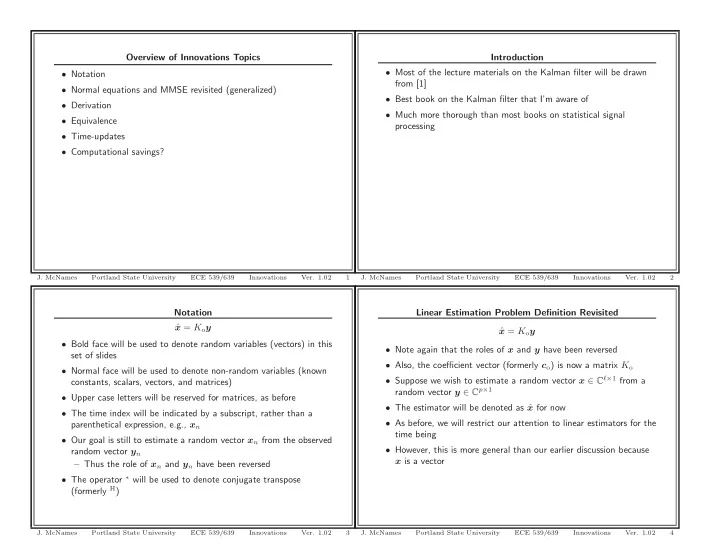
Overview of Innovations Topics Introduction • Most of the lecture materials on the Kalman filter will be drawn • Notation from [1] • Normal equations and MMSE revisited (generalized) • Best book on the Kalman filter that I’m aware of • Derivation • Much more thorough than most books on statistical signal • Equivalence processing • Time-updates • Computational savings? J. McNames Portland State University ECE 539/639 Innovations Ver. 1.02 1 J. McNames Portland State University ECE 539/639 Innovations Ver. 1.02 2 Notation Linear Estimation Problem Definition Revisited x = K o y ˆ x = K o y ˆ • Bold face will be used to denote random variables (vectors) in this • Note again that the roles of x and y have been reversed set of slides • Also, the coefficient vector (formerly c o ) is now a matrix K o • Normal face will be used to denote non-random variables (known • Suppose we wish to estimate a random vector x ∈ C ℓ × 1 from a constants, scalars, vectors, and matrices) random vector y ∈ C p × 1 • Upper case letters will be reserved for matrices, as before • The estimator will be denoted as ˆ x for now • The time index will be indicated by a subscript, rather than a • As before, we will restrict our attention to linear estimators for the parenthetical expression, e.g., x n time being • Our goal is still to estimate a random vector x n from the observed • However, this is more general than our earlier discussion because random vector y n x is a vector – Thus the role of x n and y n have been reversed • The operator ∗ will be used to denote conjugate transpose (formerly H ) J. McNames Portland State University ECE 539/639 Innovations Ver. 1.02 3 J. McNames Portland State University ECE 539/639 Innovations Ver. 1.02 4

Inner Products Problem Definition: Revisiting the MSE � x � 2 � � x , x � x ) ∗ ] = E [˜ x ∗ ] P ( K ) � E [( x − ˆ � x , y � � E [ xy ∗ ] x )( x − ˆ x ˜ x ⊥ y : � x , y � = 0 • If we have multiple outputs that we are estimating simultaneously, • The �·� notation is used to denote an inner product how do we calculate the mean squared error (MSE)? • It is unusual that our inner product is actually an (expected) outer • What if estimating some elements of x is more important than product of vectors others? • Nonetheless, all of the properties of a inner product space are • Let’s say we were interested in a linear combination of the satisfied and the projection theorem holds individual errors for each element of x : • Thus the optimal estimate is still orthogonal to the residuals z � a ∗ x (errors) z = E[ z | y ] = E[ a ∗ x | y ] = a ∗ E[ x | y ] = a ∗ ˆ � y , x − K o y � = 0 ˆ x x ) = a ∗ ˜ • Generalizes all of the solutions to any inner product space z � z − ˆ z = a ∗ ( x − ˆ ˜ x • For all of our applications just denotes the expected outer product z � 2 ] related to the error covariance • How is the minimum of E[ � ˜ of random vectors matrix P ( K ) ? J. McNames Portland State University ECE 539/639 Innovations Ver. 1.02 5 J. McNames Portland State University ECE 539/639 Innovations Ver. 1.02 6 The Error Covariance Matrix Solving the Normal Equations (again) z ∗ ] = E[( a ∗ ˜ x )( a ∗ ˜ x ) ∗ ] = a ∗ E[˜ z � 2 ] = E[˜ x ∗ ] a = a ∗ P ( K ) a P ( K ) = E [( x − K y )( x − K y ) ∗ ] E[ � ˜ z ˜ x ˜ = E[ xx ∗ ] − K E[ yx ∗ ] − E[ xy ∗ ] K ∗ + K E[ yy ∗ ] K ∗ • For any given vector a , the MSE is minimized by finding the error = R x − KR yx − R xy K ∗ + KR y K covariance matrix such that � � R x R xy � � I � � I � a ∗ P ( K ) a ≥ a ∗ P ( K o ) a a ∗ [ P ( K ) − P ( K o )] a ≥ 0 � � � = I − K = I − K R − K ∗ − K ∗ R yx R y • This means that an equivalent problem is to find K o such that Suppose R y > 0 (positive definite, invertible) then we can factor the P ( K ) − P ( K o ) is nonnegative definite for all K joint covariance matrix in uper-lower block triangular form as • The solution to this problem is independent of a ! � � � I R xy R − 1 � � � � � R x R xy R ˜ 0 I 0 x y = • Commonly denoted as P ( K ) ≥ P ( K o ) R − 1 y R yx I R yx R y 0 I 0 R y • Thus we can generalize the notion of minimizing MSE in the where vector case to mean minimize the matrix error covariance x ∗ ] P ( K ) = E[˜ x ˜ R xy = R ∗ x � R x − R xy R − 1 R ˜ y R yx yx is called the Schur complement of R x in R J. McNames Portland State University ECE 539/639 Innovations Ver. 1.02 7 J. McNames Portland State University ECE 539/639 Innovations Ver. 1.02 8

Normal Equations: Completing the Square Normal Equations: Finding the Optimal Solution Then x + ( R xy R − 1 − K ) R y ( R xy R − 1 − K ) ∗ P ( K ) = R ˜ y y − K � � � � � R x R xy I a ∗ P ( K ) a = a ∗ R ˜ x a + a ∗ ( R xy R − 1 − K ) R y ( R xy R − 1 − K ) ∗ a � I P ( K ) = − K ∗ y y R yx R y a � ( R xy R − 1 − K ) ∗ a ´ R xy R − 1 − K � � I � � � � � � � R ˜ 0 I 0 I y x � I y = P ( K ) = a ∗ R ˜ a ∗ R y ´ R − 1 − K ∗ x a + ´ a 0 I 0 R y y R yx I a ∗ R y ´ ´ a ≥ 0 for any vector ´ a �� � R ˜ � � � 0 I x � I � R xy R − 1 = − K � R − 1 y R yx − K ∗ � y P ( K ) ≥ a ∗ R ˜ 0 R y x a � � � I ( R xy R − 1 � R ˜ − K ) R y Since the final expression doesn’t depend on K , P ( K ) is minimized = x ( R xy R − 1 − K ) ∗ y y when x + ( R xy R − 1 − K ) R y ( R xy R − 1 − K ) ∗ = R ˜ K = K o � R xy R − 1 y y y = R x − R xy R − 1 y R yx + ( R xy R − 1 − K ) R y ( R xy R − 1 − K ) ∗ and the minimum error covariance matrix is y y x = R x − R xy R − 1 P ( K o ) = R ˜ y R yx = R x − R xy K o J. McNames Portland State University ECE 539/639 Innovations Ver. 1.02 9 J. McNames Portland State University ECE 539/639 Innovations Ver. 1.02 10 Normal Equations Revisited Exploiting Structure More generally, you can show that the MMSE estimator is given by • So far we have tried to estimate one random variable (formerly y , any solution of the normal equations even when R y is not invertible now x n ) from another (formerly x , now y ) • In many applications the random variables have additional K o R y = R xy structure that we can exploit These look quite different from the normal equations we obtained – More insightful solutions earlier – Can frame problem in terms of known quantities and not just the auto- and cross-correlations Rc o = d – Can reduce the computation but they become the same if we consider that we are now estimating x • Example: Stationary FIR filters from y . Suppose x is a scalar, then we can express the normal equations in a form similar to the one we worked with before: K ∗ 1 × p R y K o = R xy R y = R yx o p × p 1 × p p × p p × 1 p × 1 J. McNames Portland State University ECE 539/639 Innovations Ver. 1.02 11 J. McNames Portland State University ECE 539/639 Innovations Ver. 1.02 12