Over-parameterized nonlinear learning: Gradient descent follows the - PowerPoint PPT Presentation
Over-parameterized nonlinear learning: Gradient descent follows the shortest path? Samet Oymak and Mahdi Soltanolkotabi Department of Electrical and Computer Engineering June 2019 June 2019 Motivation Modern learning (e.g. deep learning)
Over-parameterized nonlinear learning: Gradient descent follows the shortest path? Samet Oymak and Mahdi Soltanolkotabi Department of Electrical and Computer Engineering June 2019 June 2019
Motivation Modern learning (e.g. deep learning) involves fitting nonlinear models
Motivation Modern learning (e.g. deep learning) involves fitting nonlinear models Mystery # of parameters >> # of training data
Motivation Modern learning (e.g. deep learning) involves fitting nonlinear models Mystery # of parameters >> # of training data
Motivation Modern learning (e.g. deep learning) involves fitting nonlinear models Mystery # of parameters >> # of training data
Motivation Modern learning (e.g. deep learning) involves fitting nonlinear models Mystery # of parameters >> # of training data Challenges Optimization: Why can you find a global optima despite nonconvexity? Generalization: Why is the global optima any good for prediction?
Prelude: over-parametrized linear least-squares θ ∈ R p L ( θ ) := 1 2 � Xθ − y � 2 X ∈ R n × p min with and n ≤ p. ℓ 2
Prelude: over-parametrized linear least-squares θ ∈ R p L ( θ ) := 1 2 � Xθ − y � 2 X ∈ R n × p min with and n ≤ p. ℓ 2 Gradient descent starting from θ 0 has three properties:
Prelude: over-parametrized linear least-squares θ ∈ R p L ( θ ) := 1 2 � Xθ − y � 2 X ∈ R n × p min with and n ≤ p. ℓ 2 Gradient descent starting from θ 0 has three properties: Global convergence
Prelude: over-parametrized linear least-squares θ ∈ R p L ( θ ) := 1 2 � Xθ − y � 2 X ∈ R n × p min with and n ≤ p. ℓ 2 Gradient descent starting from θ 0 has three properties: Global convergence Converges to closest global optima to θ 0
Prelude: over-parametrized linear least-squares θ ∈ R p L ( θ ) := 1 2 � Xθ − y � 2 X ∈ R n × p min with and n ≤ p. ℓ 2 Gradient descent starting from θ 0 has three properties: Global convergence Converges to closest global optima to θ 0 Follows a direct trajectory
Over-parametrized nonlinear least-squares θ ∈ R p L ( θ ) := 1 2 � f ( θ ) − y � 2 min ℓ 2 , where y 1 f ( x 1 ; θ ) y 2 f ( x 2 ; θ ) ∈ R n , ∈ R n , y := f ( θ ) := and n ≤ p. . . . . . . y n f ( x n ; θ )
Over-parametrized nonlinear least-squares θ ∈ R p L ( θ ) := 1 2 � f ( θ ) − y � 2 min ℓ 2 , where y 1 f ( x 1 ; θ ) y 2 f ( x 2 ; θ ) ∈ R n , ∈ R n , y := f ( θ ) := and n ≤ p. . . . . . . y n f ( x n ; θ ) Run gradient descent: θ τ +1 = θ τ − η τ ∇L ( θ τ )
Over-parametrized nonlinear least-squares θ ∈ R p L ( θ ) := 1 2 � f ( θ ) − y � 2 min ℓ 2 , where y 1 f ( x 1 ; θ ) y 2 f ( x 2 ; θ ) ∈ R n , ∈ R n , y := f ( θ ) := and n ≤ p. . . . . . . y n f ( x n ; θ ) Run gradient descent: θ τ +1 = θ τ − η τ ∇L ( θ τ ) Gradient and Jacobian ∇L ( θ ) = J ( θ ) T ( f ( θ ) − y ) . ∈ R n × p is the Jacobian matrix J ( θ ) = ∂f ( θ ) ∂ θ Intuition: Jacobian replaces the feature matrix X
Gradient descent trajectory Assumptions minimum singular value at initialization: σ min ( J ( θ 0 )) ≥ 2 α maximum singular value: �J ( θ ) � ≤ β Jacobian smoothness: �J ( θ 2 ) − J ( θ 1 ) � ≤ L � θ 2 − θ 1 � ℓ 2 Initial error: � f ( θ 0 ) − y � ℓ 2 ≤ α 2 4 L
Gradient descent trajectory Assumptions minimum singular value at initialization: σ min ( J ( θ 0 )) ≥ 2 α maximum singular value: �J ( θ ) � ≤ β Jacobian smoothness: �J ( θ 2 ) − J ( θ 1 ) � ≤ L � θ 2 − θ 1 � ℓ 2 Initial error: � f ( θ 0 ) − y � ℓ 2 ≤ α 2 4 L Theorem (Oymak and Soltanolkotabi 2018) � f ( θ 0 ) − y � ℓ 2 1 Assume above over a ball of radius R = around θ 0 and Set η = β 2 . α Global convergence: � τ α 2 � 1 − 1 � f ( θ τ ) − y � 2 � f ( θ 0 ) − y � 2 ℓ 2 ≤ ℓ 2 2 β 2 Converges to near closest global minima to initialization: � θ τ − θ 0 � ℓ 2 ≤ β α � θ ∗ − θ 0 � ℓ 2 Takes an approximately direct route
Concrete example: One-hidden layer neural net Training data: ( x 1 , y 1 ) , ( x 2 , y 2 ) , . . . , ( x n , y n ) Loss: � 2 v T φ ( W x i ) − y i L ( v , W ) := � n � i =1 Algorithm: gradient descent with random Gaussian initialization Theorem (Oymak and Soltanolkotabi 2019) As long as # parameters � (# of training data ) 2 Then, with high probability Zero training error: L ( v τ , W τ ) ≤ (1 − ρ ) τ L ( v 0 , W 0 ) Iterates remain close to initialization
Further results and applications Extensions to SGD and other loss functions Theoretical justification for Early stopping Generalization Robustness to label noise Other applications Fitting generalized Low-rank matrix recovery linear models
Conclusion (Stochastic) gradient descent has three intriguing properties Global convergence Converges to near closest global optima to init. Follows a direct trajectory
Thanks! Poster Thursday, 6:30 PM, # 95 References Over-parametrized nonlinear learning: Gradient descent follows the shortest path? S. Oymak and M. Soltanolkotabi Towards moderate overparameterization: global convergence guarantees for training shallow neural networks. S. Oymak and M. Soltanolkotabi Gradient Descent with Early Stopping is Provably Robust to Label Noise for Overparameterized Neural Networks. M. Li, M. Soltanolkotabi, and S. Oymak Generalization Guarantees for Neural Networks via Harnessing the Low-rank Structure of the Jacobian. S. Oymak, Z. Fabian, M. Li, and M. Soltanolkotabi
Recommend
More recommend
Explore More Topics
Stay informed with curated content and fresh updates.

