{ output 1 if a q . y = 0 if a < q w n x n 3 1 9/27/2016 - PowerPoint PPT Presentation
9/27/2016 Classification INF3490 - Biologically inspired computing Lecture 28th September 2016 DOG Trained Classifier Multi-Layer Neural Networks Kai Olav Ellefsen Perceptron Training a classifier (supervised learning) inputs x 1
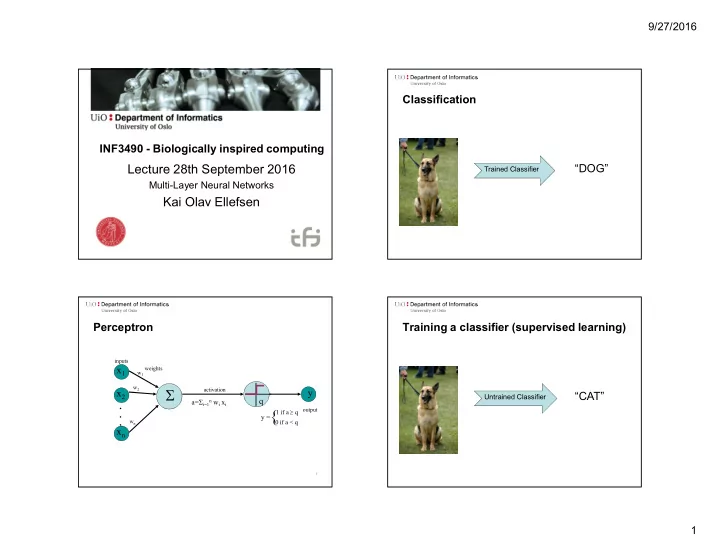
9/27/2016 Classification INF3490 - Biologically inspired computing Lecture 28th September 2016 “DOG” Trained Classifier Multi-Layer Neural Networks Kai Olav Ellefsen Perceptron Training a classifier (supervised learning) inputs x 1 weights w 1 w 2 activation y x 2 “CAT” Untrained Classifier a= i=1n w i x i q . . { output 1 if a q . y = 0 if a < q w n x n 3 1
9/27/2016 Training a classifier (supervised learning) Training a perceptron inputs x 1 weights w 1 w 2 activation x 2 y . a= i=1n w i x i q . { output 1 if a q “CAT” Untrained Classifier . y = 0 if a < q w n x n No, it was a dog. Adjust classifier parameters 6 Decision Surface A Quick Overview 1 1 Decision line • Linear Models are easy to understand. x 2 w 1 x 1 + w 2 x 2 = q 1 • However, they are very simple. 0 0 – They can only identify flat decision boundaries 0 (straight lines, planes, hyperplanes, ...). x 1 1 • Majority of interesting data are not linearly 0 0 separable. Then? 7 8 2
9/27/2016 A Quick Overview Multi-Layer Perceptron (MLP) • Learning in the neural networks (NN) happens in -1 -1 Input Layer the weights. • Weights are associated with connections. Hidden Layer Output Layer • Thus, it is sensible to add more connections to perform more complex computations. • Two ways for non-lin. separation (not exclusive): – Recurrent Network : connect the output neurons to the inputs with feedback connections. – Multi-layer perceptron network : add neurons between the input nodes and the outputs. 9 10 Solution for XOR : Add a Hidden Layer !! XOR Problem Minsky & Papert (1969) offered solution to XOR problem by combining perceptron unit responses using a second layer of units . +1 XOR (Exclusive OR) Problem 1 3 Perceptron does not work here. 2 Single layer generates a linear decision boundary. +1 12 11 3
9/27/2016 XOR Again XOR Again E E Output -0.5 -0.5 -1 1 -1 A B C in C out D in D out E in 1 C D Hidden Layer 0 0 -0.5 0 -1 0 -0.5 C D -0.5 -0.5 -1 -1 0 1 0.5 1 0 0 0.5 1 1 1 1 1 1 1 1 A B Inputs A B 1 0 0.5 1 0 0 0.5 1 1 1.5 1 1 1 -0.5 13 Multilayer Network Structure MLP Decision Boundary – Nonlinear Problems, Solved! • A neural network with one or more layers of nodes between the input and the output nodes is called multilayer network . In contrast to perceptrons, multilayer networks can learn not • The multilayer network structure , or architecture , or topology , only multiple decision boundaries, but the boundaries may consists of an input layer , one or more hidden layers , and one also be nonlinear. output layer . X 2 • The input nodes pass values to the first hidden layer, its nodes to the second and so until producing outputs. • A network with a layer of input units, a layer of hidden units and a layer of output units is a two-layer network . • A network with two layers of hidden units is a three- layer network , and so on. Internal nodes Output nodes Input nodes X 1 15 16 4
9/27/2016 Properties of the Multi-Layer How to Train MLP? Perceptron • How we can train the network, so that • No connections within a single layer. – The weights are adapted to generate correct (target • No direct connections between input and output answer)? x 1 (t j - y j ) layers. • Fully connected; all nodes in one layer connect to all • In Perceptron, errors are computed at the output. nodes in the next layer. • In MLP, • Number of output units need not equal number of input units. – Don ’ t know which weights are wrong: • Number of hidden units per layer can be more or less – Don ’ t know the correct activations for the neurons in the hidden layers. than input or output units. 18 Backpropagation Then… Rumelhart, Hinton and Williams (1986) ( though actually invented earlier in a PhD thesis relating to economics) The problem is : How to train Multi Layer y j d j Backward step: Perceptrons?? propagate errors from w jk output to hidden layer Solution : Backpropagation Algorithm (Rumelhart and colleagues,1986) x k d k w ki Forward step: Propagate activation x i from input to output layer 19 5
9/27/2016 Training MLPs Training MLPs Forward Pass Backward Pass 1. Put the input values in the input layer. 1. Calculate the output errors 2. Calculate the activations of the hidden nodes. 2. Update last layer of weights. 3. Calculate the activations of the output nodes. 3. Propagate error backward, update hidden weights. 4. Until first layer is reached. 21 22 Back Propagation Algorithm Error Function • The backpropagation training algorithm uses the gradient descent technique to minimize • Single scalar function for entire network. the mean square difference between the • Parameterized by weights (objects of interest). desired and actual outputs. • Multiple errors of different signs should not cancel out. • The network is trained initially selecting small • Sum-of-squares error: random weights and then presenting all training data incrementally. • Weights are adjusted after every trial until they converge and the error is reduced to an acceptable value . 23 24 6
9/27/2016 Gradient Descent Error Terms E • Need to differentiate the error function • The full calculation is presented in the book. • Gives us the following error terms (deltas) • For the outputs d ( y t ) g ' ( a ) k k k k w • For the hidden nodes d d g ' ( u ) w i i k ik k 25 26 BackPropagation Algorithm Update Rules • This gives us the necessary update rules • For the weights connected to the outputs: y 1 x 1 e 1 d w w z x 2 y 2 E jk jk k j e 2 ( X , T ) X x 3 Y y 3 • For the weights on the hidden nodes: e 3 x 4 T d v v x y 4 x 5 e 4 ij ij j i • The learning rate depends on the application. Values between 0.1 and 0.9 have been used in many applications. 27 28 7
9/27/2016 Example: Backpropagation Algorithm (sequential) 1. Apply an input vector and calculate all activations, a and u 2. Evaluate deltas for all output units: d ( y t ) g ' ( a ) v 11 = -1 k k k k x 1 w 11 = 1 y 1 3. Propagate deltas backwards to hidden layer deltas: v 12 = 0 w 12 = -1 d d g ' ( u ) w i i k ik v 21 = 0 w 21 = 0 k x 2 y 2 v 22 = 1 4. Update weights: w 22 = 1 v 01 = 1 d w w z v 02 = 1 jk jk k j d v v x Use identity activation function (ie g(a) = a) for simplicity of example ij ij j i 30 Example: Backpropagation Example: Backpropagation Forward pass. Calculate 1 st layer activations: All biases set to 1. Will not draw them for clarity. Learning rate h = 0.1 u 1 = 1 v 11 = -1 x 1 = 0 w 11 = 1 v 11 = -1 y 1 x 1 = 0 x 1 w 11 = 1 y 1 v 12 = 0 w 12 = -1 v 12 = 0 w 12 = -1 v 21 = 0 w 21 = 0 v 21 = 0 y 2 w 21 = 0 x 2 = 1 v 22 = 1 x 2 = 1 x 2 y 2 v 22 = 1 w 22 = 1 w 22 = 1 u 2 = 2 Have input [0 1] with target [1 0]. u 1 = -1x0 + 0x1 +1 = 1 u 2 = 0x0 + 1x1 +1 = 2 31 32 8
9/27/2016 Example: Backpropagation Example: Backpropagation Calculate 2 nd layer outputs (weighted sum through activation Calculate first layer outputs by passing activations through activation functions functions): z 1 = 1 z 1 = 1 v 11 = -1 v 11 = -1 x 1 w 11 = 1 x 1 w 11 = 1 y 1 y 1 = 2 v 12 = 0 v 12 = 0 w 12 = -1 w 12 = -1 v 21 = 0 v 21 = 0 w 21 = 0 w 21 = 0 x 2 y 2 v 22 = 1 x 2 y 2 = 2 z 2 = 2 v 22 = 1 w 22 = 1 w 22 = 1 z 2 = 2 y 1 = a 1 = 1x1 + 0x2 +1 = 2 z 1 = g(u 1 ) = 1 y 2 = a 2 = -1x1 + 1x2 +1 = 2 z 2 = g(u 2 ) = 2 33 34 Example: Backpropagation Example: Backpropagation Backward pass : Calculate weight changes for 1 st layer: d ( y t ) g ' ( a ) z 1 = 1 k k k k v 11 = -1 d 1 z 1 =-1 x 1 w 11 = 1 v 11 = -1 x 1 w 11 = 1 d 1 = 1 v 12 = 0 d 1 z 2 =-2 w 12 = -1 v 12 = 0 v 21 = 0 w 12 = -1 w 21 = 0 v 21 = 0 d 2 z 1 =-2 x 2 v 22 = 1 w 21 = 0 d 2 = 2 x 2 v 22 = 1 w 22 = 1 d 2 z 2 =-4 w 22 = 1 z 2 = 2 Target =[1, 0] so t 1 = 1 and t 2 = 0. So: d w w z d 1 = (y 1 - t 1 )= 2 – 1 = 1 d 2 = (y 2 - t 2 )= 2 – 0 = 2 jk jk k j 35 36 9
9/27/2016 Example: Backpropagation Example: Backpropagation Weight changes will be : Calculate hidden layer deltas : v 11 = -1 v 11 = -1 D 1 w 11 = 1 x 1 x 1 w 11 = 0.9 D 1 = 1 v 12 = 0 v 12 = 0 w 12 = -1.2 D 2 w 12 = -2 v 21 = 0 v 21 = 0 D 1 w 21 = 0 w 21 = -0.2 D 2 = 2 x 2 x 2 v 22 = 1 v 22 = 1 w 22 = 0.6 D 2 w 22 = 2 d w w z d D g ' ( u ) w jk jk k j i i k ik k 37 38 Example: Backpropagation Example: Backpropagation Deltas propagate back: d D g ' ( u ) w i i k ik And are multiplied by inputs : k d 1 x 1 = 0 d 1 = -1 v 11 = -1 x 1 = 0 v 11 = -1 x 1 D 1 = -1 D 1 = 1 v 12 = 0 d 1 x 2 = 1 v 12 = 0 v 21 = 0 v 21 = 0 d 2 x 1 = 0 D 2 = -2 x 2 = 1 D 2 = 2 v 22 = 1 x 2 v 22 = 1 d 2 x 2 = -2 d 2 = 2 d 1 = 1 - 2 = -1 d v v x d 2 = 0 + 2 = 2 ij ij j i 39 40 10
Recommend
More recommend
Explore More Topics
Stay informed with curated content and fresh updates.

