Optimal estimation of certain random quantities Mark Podolskij Risk - PowerPoint PPT Presentation

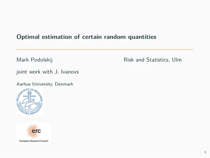
Optimal estimation of certain random quantities Mark Podolskij Risk and Statistics, Ulm joint work with J. Ivanovs Aarhus University, Denmark 1

Topic of the talk Let ( X t ) t ∈ [0 , 1] be a stochastic process (Brownian motion, Lévy process, SDE etc.). Given the observations X 0 , X ∆ n , X 2∆ n , . . . , X ⌊ 1 / ∆ n ⌋ ∆ n with ∆ n → 0 and the random parameter of interest Q , what is the optimal estimator of Q ? 2

Low vs. high frequency data Low frequency data High frequency data Observed data Observed data X 0 ( ω ) , X ∆ n ( ω ) , ..., X ⌊ 1 / ∆ n ⌋ ∆ n ( ω ) X 1 , X 2 , ..., X n i . i . d . ∼ F Asymptotic knowledge Asymptotic knowledge ( X t ( ω )) t ∈ [0 , 1] distribution function F Identifiable objects Identifiable objects functionals of ( X t ( ω )) t ∈ [0 , 1] functionals of F 3

Background � In the classical test theory the model parameters are deterministic objects. There exist numerous approaches to access the optimality of estimators: Cramer-Rao bounds, maximum likelihood theory, minimax approach, Le Cam theory, etc. � However, in the high frequency setting the objects of interests are often random . Examples include quadratic variation, realised jumps, supremum/infimum of a process, local times, occupation time measures etc. � In this framework very little is known about how to construct optimal estimates. 4

Example: Estimation of the quadratic variation Let X be a continuous semimartingale of the form � t � t t ≥ 0 X t = X 0 + a s ds + σ s dW s 0 0 where a and σ are stochastic processes, and W is a Brownian motion. An important result in the theory of high frequency data is the following theorem. Theorem (Jacod(94)) It holds that   � 1 � � 1 � ⌊ 1 / ∆ n ⌋ � � � 2 −  d st ∆ − 1 / 2  σ 2 σ 4 X i ∆ n − X ( i − 1)∆ n s ds → MN 0 , 2 s ds n 0 0 i =1 Recently, Clement, Delattre & Gloter (13) have proved that the above estimator is asymptotically efficient applying an infinite dimensional LAMN property. 5

Introduction � The results of Clement, Delattre & Gloter (13) only cover estimation problems for volatility functionals. In this talk we will rather focus on the following random objects: X := sup X s s ∈ [0 , 1] � 1 1 l ( x ) := lim 1 ( − ǫ,ǫ ) ( X s − x ) ds 2 ǫ ǫ ↓ 0 0 � 1 L ( x ) := 1 ( x , ∞ ) ( X s ) ds 0 which is the supremum, local time and occupation time measure of the process X , respectively. � We are interested in optimal estimation of these objects given high frequency data ( X i ∆ n ) 0 ≤ i ≤⌊ 1 / ∆ n ⌋ . 6

A remark on optimality We will see that many naive estimators are rate optimal, but not efficient! In fact, efficient estimators are easy to introduce. Let Q = Φ(( X s ) s ∈ [0 , 1] ) be a random variable of interest. An optimal estimator of Q is given as (i) in L 2 -sense: E [ Q | ( X i ∆ n ) 0 ≤ i ≤⌊ 1 / ∆ n ⌋ ] (ii) in L 1 -sense: median[ Q | ( X i ∆ n ) 0 ≤ i ≤⌊ 1 / ∆ n ⌋ ] We will investigate the asymptotic theory for these type of estimates in the setting of supremum, local time and occupation time measure of the process X , where X is a Brownian motion, stable Lévy process or a continuous diffusion process. 7

Naive estimator of the supremum � It is rather simple to propose the following estimate for the supremum P M n := i =1 ,..., ⌊ 1 / ∆ n ⌋ X i ∆ n max → X where the consistency holds for all Lévy processes X . � The asymptotic theory for the maximum has been studied in several papers including Asmussen, Glynn & Pitman (95) (Brownian motion) and Ivanovs (18) (general Lévy processes). � Since M n < X , the estimator M n is downward biased and there were several attempts to correct the bias. 8

A result on zooming-in at supremum The following result from the theory of Lévy processes will be extremely useful for our asymptotic theory. Theorem (Ivanovs (18)) Let X be an α -stable Lévy process with α ∈ (0 , 2] . Denote by τ the time of the supremum of X on the interval [0 , 1] . Then we obtain the functional stable convergence � � � � d st � ( Z n ∆ − 1 /α ( X τ + t ∆ n − X τ ) → t ) t ∈ R := X t n t ∈ R t ∈ R where � X is the so called Lévy process conditioned to stay negative , which is independent of F . When X is a Brownian motion, we deduce the identity � X t = −� B t � where B is a 3 -dimensional Brownian motion. 9

Application to estimation of the supremum The previous result has the following consequence. Theorem (Ivanovs (18)) Let X be an α -stable Lévy process with α ∈ (0 , 2] . Then it holds that � � d j ∈ Z ( � ∆ − 1 /α M n − X → max X j + U ) n where U ∼ U (0 , 1) is independent of � X and F . Sketch of proof: Note that � � ∆ − 1 /α = Z n X ( ⌈ τ/ ∆ n ⌉ + i )∆ n − X τ n i + { τ/ ∆ n } → U ∼ U (0 , 1). Since Z n d st d st → � Recall that { τ/ ∆ n } X , we conclude that � � d j ∈ Z ( � ∆ − 1 /α M n − X → max X j + U ) n ✷ 10

Computation of the optimal estimator: The Brownian case The basis of our approach is the computation of the conditional probability � � H n ( x ) := P X ≤ x | ( X i ∆ n ) 0 ≤ i ≤⌊ 1 / ∆ n ⌋ x > 0 . Due to Markov and self-similarity property of X , we easily see that � � � n ∆ − 1 / 2 n ) , ∆ − 1 / 2 ∆ n H n ( x ) = ( x − X i − 1 F i X n n i =1 � � where F ( x , y ) = P X ≤ x | X 1 = y = 1 − exp( − 2 x ( x − y )). After rescaling we deduce the stable convergence � � � � � ∆ 1 / 2 x + ∆ − 1 / 2 ( M n − X ( i − 1)∆ n ) , ∆ − 1 / 2 ∆ n H n x + M n = F i X n n n i ∈ Z � � � d st X j + U − � � X i + U , � X i +1+ U − � → G ( x ) := x + max . F X i + U j ∈ Z i ∈ Z 11

Conditional mean and conditional median � � � For the conditional mean T (2) := E X | ( X i ∆ n ) i we obtain the n formula � ∞ � � �� T (2) − X = ( M n − X ) + ∆ 1 / 2 ∆ 1 / 2 1 − H n x + M n dx n n n 0 Hence, the probabilistic structure of X only affects the second order term. � � � Similarly, for the conditional median T (1) X | ( X i ∆ n ) i := median we n deduce the identity � � − 1 T (1) − X = ( M n − X ) + ∆ 1 / 2 ∆ 1 / 2 H n · + M n (1 / 2) n n n and again the probabilistic structure of X only affects the second order term. 12

Asymptotic theory for the optimal estimators: Brownian case Theorem (Ivanovs & P. (19)) Define the estimates � � � � T (1) T (2) X | ( X i ∆ n ) i X | ( X i ∆ n ) i = median , = E . n n (i) It holds that � � d j ∈ Z ( � ∆ − 1 / 2 T (1) X j + U ) + G − 1 (1 / 2) . − X → max n n (ii) Furthermore, � ∞ � � d j ∈ Z ( � ∆ − 1 / 2 T (2) − X → max (1 − G ( y )) dy . X j + U ) + n n 0 In particular, we have that MSE ( M n ) ≈ 6 . 25 ! MSE ( T (2) n ) 13

Simulation of asymptotic distributions 1.5 1.0 type density conditional expectation conditional median old 0.5 0.0 0 1 2 error 14

Asymptotic theory: The α -stable case Theorem (Ivanovs & P. (19)) Let X be a α -stable Lévy motion with α ∈ (0 , 2) . (i) Define T (1) = median [ X | ( X i ∆ n ) i ] . Then we obtain n � � d j ∈ Z ( � ∆ − 1 /α T (1) X j + U ) + G − 1 (1 / 2) . − X → max n n and the estimator is L 1 -optimal for α ∈ (1 , 2) . (ii) Define T (2) = E [ X | ( X i ∆ n ) i ] for α ∈ (1 , 2) . Then it holds that n � ∞ � � d j ∈ Z ( � ∆ − 1 /α T (2) − X → max X j + U ) + (1 − G ( y )) dy . n n 0 15

Naive estimators for the local time � In this chapter we assume that X is a Brownian motion. Recall the definition of local time: � 1 1 l ( x ) = lim 1 ( − ǫ,ǫ ) ( X s − x ) ds 2 ǫ ǫ ↓ 0 0 where x ∈ R . � A straightforward estimator of l ( x ) is given as ⌊ 1 / ∆ n ⌋ � P l n ( x ) := a n ∆ n g ( a n ( X i ∆ n − x )) → l ( x ) i =1 � where g is a kernel satisfying R g ( x ) dx = 1, and a n → ∞ with a n ∆ n → 0. � We will focus on a more general class of statistics: ⌊ 1 / ∆ n ⌋ � � � V ( h , x ) n := a n ∆ n a n ( X i ∆ n − x ) , ∆ − 1 / 2 ∆ n h i X n i =1 16

Asymptotic theory for V ( h , x ) n Theorem (Borodin (86), Jacod (98)) Assume that a n = ∆ − 1 / 2 and h satisfies the condition n � R | y | p h 1 ( y ) dy < ∞ for | h ( y , z ) | ≤ h 1 ( y ) exp( λ | z | ) for some λ > 0 and some p > 3 . Then it holds that P V ( h , x ) n → c h l ( x ) � �� � where c h = R h ( y , z ) ϕ ( z ) dz dy and ϕ denotes the density of the R standard normal distribution. Furthermore, we obtain the stable convergence ( V ( h , x ) n − c h l ( x )) d st ∆ − 1 / 4 → MN (0 , v h l ( x )) n for a certain constant v h > 0 . An interesting example is the number of crossings at level 0 which corresponds to x = 0 and h ( y , z ) = 1 ( −∞ , 0) ( y ( y + z )). 17