Optimal Control McGill COMP 765 Oct 3 rd , 2017 Classical Control - PowerPoint PPT Presentation
Optimal Control McGill COMP 765 Oct 3 rd , 2017 Classical Control Quiz Question 1: Can a PID controller be used to balance an inverted pendulum: A) That starts upright? B) That must be swung - up (perhaps with multiple swings
Optimal Control McGill COMP 765 Oct 3 rd , 2017
Classical Control Quiz • Question 1: Can a PID controller be used to balance an inverted pendulum: • A) That starts upright? • B) That must be “swung - up” (perhaps with multiple swings required) • Question 2: Define: • A) Controllability • B) Stability • C) Feedback-linear • D) Under-actuated • Question 3: What is bang-bang control? Give one example where this is an optimal solution.
Review from last week • PID control laws allow manual tuning of a feedback system • Provides a way to drive the system to a “correct” state or path and stabilize it with tunable properties. • Widely used for simple systems up to self-driving cars and airplane autopilots • PID not typically used for complex behaviours: e.g, swing-up, walking and manipulation. Why?
Plan for this week • Dive into increasingly “intelligent” control strategies • Less tuning required • Start with simple known models, then complex but known, learned models in a few weeks • More complex behaviors achievable • Today’s goals: • Define optimal control • Value Iteration • Linear Quadratic Regulator
Robotic Control
From my research
Double Integrator Example • Goal: arrive at x=0 as soon as possible • Control a(t)=u, limited to |u|<=1 • Ideally solve over all x(0), v(0) x • Dynamics: u • v(t) = v(0) + ut 2 • x(t) = x(0) + v(0)t + 0.5t 0 • Cost (min-time): • g(x,u) = 0 if goal, else 1 • What is the intuitive solution?
The phase diagram of a 2 nd order 1D actuator
Solving for the time-optimal path to goal • One approach: code your intuition as a reference trajectory and utilize PID to stabilize the system around this. • This works well, but has little “intelligence” • We need algorithms that automatically “discover” this solution, as well as those for more complex robots where we have no intuition. • This is optimal control , a beautiful subject that draws inspiration from Gauss, Newton and a long string of brilliant roboticists!!!
The big idea • Optimal control involves specifying a system: • States: 𝑦 𝑢 • Actions generated by a policy: 𝑣 𝑢 = 𝜌(𝑦 𝑢−1 , 𝑣 𝑢−1 ) • Motion model : 𝑦 𝑢 = 𝑔(𝑦 𝑢−1 , 𝑣 𝑢−1 ) • Reward: 𝑠 𝑢 = (𝑦 𝑢 , 𝑣 𝑢 ) (NOTE: equivalent if this is a cost 𝑑 𝑢 = (𝑦 𝑢 , 𝑣 𝑢 ) ) • Optimal control algorithms solve for a policy that optimizes reward, either over a finite or fixed horizon • max 𝜌 𝑢 (𝑦 𝑢 , 𝑣 𝑢 ) 𝑡. 𝑢. 𝑦 𝑢 = 𝑔(𝑦 𝑢−1 , 𝑣 𝑢−1 ) , 𝑣 𝑢 = 𝜌(𝑦 𝑢−1 , 𝑣 𝑢−1 )
Optimal Control vs Reinforcement Learning • What is the difference? • There is none, formally. Several differences in culture only: • In RL it is more common to assume reward function is not known. • Solving for a policy from a known reward called “planning” in Markov Decision Processes. • RL traditionally thought about discretized problems while Optimal Control considered continuous. This is now much more mixed on both sides. • References and background material: • Doina Precup’s course on RL • Sutton and Barto book “Reinforcement Learning”
Does an optimal policy exist? • Yes, proven in idealized cases: • Hamilton-Jacobi-Bellman sufficient condition for optimality: • 𝑊 𝑦 𝑢 , 𝑢 = max 𝑣 𝑊 𝑦 𝑢+1 , 𝑢 + 1 + (𝑦 𝑢 , 𝑣 𝑢 ) • This is the “Value Function” that describes the cost -to-go from any point and allows us to decompose the global solution. Pair with Dynamic Programming to solve everywhere. • Pontryagin’s minimum principle: • H 𝑦 𝑢 , 𝑣 𝑢 , 𝜇 𝑢 , 𝑢 = 𝜇 𝑢 𝑔 𝑦 𝑢 , 𝑣 𝑢 − (𝑦 𝑢 , 𝑣 𝑢 ) • “Hamiltonian” is formed by representing dynamics constraints using Lagrange multipliers • The optimal controller minimizes the Hamiltonian (with 3 additional constraints not shown for completeness)
Historical notes • Maximum principles and the calculus of variations • Important variational principles from early roboticists: • Gauss – the principle of least action • Euler and Lagrange – equations of analytical mechanics • Hamilton – characterization using energy representation • The difficulty is fitting this into our noisy, active Tautochrone curve: Time to bottom is independent of robot systems starting point!
Classes of optimal control systems • Linear motion, Quadratic reward, Gaussian noise: • Solved exactly and in closed form over all state space by “Linear Quadratic Regulator” (LQR). One of the two big algorithms in control (along with EKF). • Non-linear motion, Quadratic reward, Gaussian noise: • Solve approximately with a wide array of methods including iLQR/DDP, another application of linearization. KF is to EKF as LQR is to iLQR/DDP. • Still a very active research topic. • Unknown motion model, non-Gaussian noise: • State-of-the- art research that includes some of the most “physically intelligent” systems existing today.
An algorithmic look at optimal control • Same naïve approach we used for localization: discretize all space • Form a grid over the cross-product of: • State dimensions • Control dimensions • Controllers must perform well globally, but Bellman’s equation tells us how to decompose and compute local solutions! • This is known as Value Iteration and is a core algorithm of Optimal Control and Reinforcement Learning
Value Iteration Pseudo-code • Initialize value function V(x) arbitrarily for all x • Repeat until converged: • For each state: • Update values: V(x) = max over actions, expected local cost plus discounted next value • For each state: • Set optimal policy to the one which locally maximizes expected local cost plus discounted next value
VI discussion • Is it guaranteed to converge? Will it converge to the optimal value? • What problems can be solved with this method? • What are its limitations? • So, when would we use it in robotics?
An alternative approach, LQR • VI decomposes space and computes local approximations, but of course we would rather have a closed-form mathematical solution that works everywhere. Is this possible? • Yes, with the same assumptions used in the EKF! • Claim: A globally optimal controller exists for the simple linear system. It is a linear control of the form 𝑣 = 𝐿 ∗ 𝑦 𝑢 • Do you believe this? What will I have to show you to prove this statement?
LQR : Outline • Proof by construction for finite horizon case • Discussion of infinite horizon case, introduce Ricatti Equations • Algorithm discussion: How can we solve for this controller in practice?
An analytical approach: LQR • Linear quadratic regulator is an example of exact analytical solution • Idea: what can we determine if the dynamics model is known and linear and the cost is quadratic Square matrices Q and R must be symmetric positive definite (spd): i.e. positive cost for ANY nonzero state or control vector
Finite-Horizon LQR • Idea: finding controls is an optimization problem • Compute the control variables that minimize the cumulative cost
Finding the LQR controller in closed-form by recursion • Let denote the cumulative cost-to-go starting from state x and moving for n time steps. • i.e. cumulative future cost from now till n more steps • is the terminal cost of ending up at state x, with no actions left to do. Let’s denote it Q: What is the optimal cumulative cost-to-go function with 1 time step left?
Finding the LQR controller in closed-form by recursion Bellman update (a.k.a. Dynamic Programming)
Finding the LQR controller in closed-form by recursion Q: How do we optimize a multivariable function with respect to some variables (in our case, the controls)?
Finding the LQR controller in closed-form by recursion
Finding the LQR controller in closed-form by recursion
Finding the LQR controller in closed-form by recursion Quadratic Quadratic Linear term in u term in u term in u A: Take the partial derivative w.r.t. controls and set it to zero. That will give you a critical point.
Finding the LQR controller in closed-form by recursion From calculus/algebra: The minimum is attained at: If M is symmetric: Q: Is this matrix invertible? Recall R, Po are positive definite matrices.
Finding the LQR controller in closed-form by recursion The minimum is attained at: So, the optimal control for the last time step is: Linear controller in terms of the state
Finding the LQR controller in closed-form by recursion The minimum is attained at: So, the optimal control for the last time step is: We computed the location of the minimum. Now, plug it back in and compute the minimum value
Finding the LQR controller in closed-form by recursion Q: Why is this a big deal? A: The cost-to-go function remains quadratic after the first recursive step.
Finding the LQR controller in closed-form by recursion … In fact the recursive steps generalize
Finite-Horizon LQR: algorithm summary // n is the # of steps left for n = 1…N with cost-to-go Optimal controller for i-step horizon is
Recommend
More recommend
Explore More Topics
Stay informed with curated content and fresh updates.
