Optimal control of re-entrant manufacturing systems Matthias Kawski - PowerPoint PPT Presentation
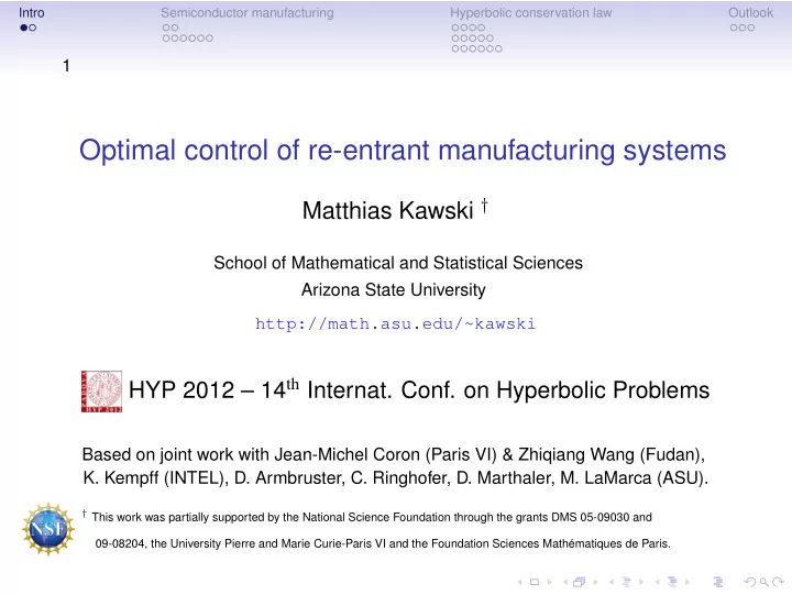
Intro Semiconductor manufacturing Hyperbolic conservation law Outlook 1 Optimal control of re-entrant manufacturing systems Matthias Kawski School of Mathematical and Statistical Sciences Arizona State University
Intro Semiconductor manufacturing Hyperbolic conservation law Outlook 1 Optimal control of re-entrant manufacturing systems Matthias Kawski † School of Mathematical and Statistical Sciences Arizona State University http://math.asu.edu/~kawski HYP 2012 – 14 th Internat. Conf. on Hyperbolic Problems Based on joint work with Jean-Michel Coron (Paris VI) & Zhiqiang Wang (Fudan), K. Kempff (INTEL), D. Armbruster, C. Ringhofer, D. Marthaler, M. LaMarca (ASU). † This work was partially supported by the National Science Foundation through the grants DMS 05-09030 and 09-08204, the University Pierre and Marie Curie-Paris VI and the Foundation Sciences Mathématiques de Paris.
Intro Semiconductor manufacturing Hyperbolic conservation law Outlook Outline • Semiconductor manufacturing Some background and mathematical problems • A hyperbolic conservation law ∂ t ρ ( t , x ) + ∂ x ( λ ( W ( t )) ρ ( t , x )) = 0 � 1 1 W ( t ) = ρ ( t , x ) dx , later specialize to λ ( W ) = 1 + W 0 • Motivation • Intuitive properties, numerical studies • Analysis: existence[ZW], optimality, L 1 vs L 2 , minimum-time • More control problems under investigation
Intro Semiconductor manufacturing Hyperbolic conservation law Outlook Selected immediately related references • D. Armbruster, D. Marthaler, C. Ringhofer, K. Kempf, and T.-C. Jo, A Continuum Model For A Re-Entrant Factory , Oper. Res., 54 (2006), 933–950. • M. La Marca, D. Armbruster, M. Herty, and C. Ringhofer, Control of continuum models of production systems, IEEE Trans. Automat. Control 55 (2010), no. 11, 2511–2526. • J.-M. Coron, M. Kawski, and Z. Wang, Analysis of a conservation law modeling a highly re-entrant manufacturing system , Discrete Contin. Dyn. Syst. Ser. B 14 (2010), no. 4, 1337–1359. • R. Colombo, M. Herty, and M. Mercier, Control of the continuity equation with a non local flow , ESAIM Control Optim. Calc. Var., 17 (2011), no. 2, 353–379. • vast body of related literature
Intro Semiconductor manufacturing Hyperbolic conservation law Outlook Semiconductor manufacturing: Distinguishing features • Product: small size, high value, global supply network • Volatile demand, difficult to predict yields (processor speed, energy consumption, . . . ). Stochastics everywhere • Typical 20 day pure processing time, 60 day start2finish, compare to demand forecast horizon • Very short product life times, never in equilibrium • New “fab” every few years & huge capital cost, utilization • Layered (sandwich) structure: highly re-entrant manufacturing line (e.g., 600 processes, 200 stations)
Intro Semiconductor manufacturing Hyperbolic conservation law Outlook Supply chains, collaboration ASU and INTEL • Several new fabs in Chandler, AZ • 90s: scheduling processes/machines. E.g., chaos, queuing models, discrete event systems. • Hierarchical control, inner-outer-loop, “model predictive” • 2000: global supply network, many products • “downbinning” – stochastic optimal control • early 2000s: fast computation using PDE models compare gas dynamics, traffic flow. (K.Kempff (INTEL), D.Armbruster, C.Ringhofer, D.Marthaler, M.LaMarca, . . . )
Intro Semiconductor manufacturing Hyperbolic conservation law Outlook Toy example: M sets of machines, N processing steps C, D ✐ ✐ A, B 1 2 ✲ ✲ ✐ ✐ ✓✏ ✓✏ ✓✏ ✓✏ ✓✏ ✓✏ ✄� A, B C, D ✲ 3 ✲ 4 ✲ ✲ ✲ ✲ ✲ ✲ ✲ ✐ ✐ 1 2 3 4 5 6 ✄�✄� 5 6 ✒✑ ✒✑ ✒✑ ✒✑ ✒✑ ✒✑ ✲ ✲ ✲ ✄� ✛ ✛ The machine-based view The process-based view Real world • approx N ≈ 600 production steps total, up to 20 loops • approx M ≈ 200 work-stations, up to 20 parallel machines • total processing time approximately 20 days • total manufacturing time approximately 60 days • several different products (common: shared initial steps)
Intro Semiconductor manufacturing Hyperbolic conservation law Outlook Sample data for toy example: queues and idling Topology M machines N process steps. � 1 � 1 Φ = ( p ij ) where p ij = 1 if machine i can ∈ R 200 × 600 Φ= 1 1 carry out process j , and p ij = 0 else. Process times τ ij is the time it takes ma- � 11 � 17 chine i to complete process step j . τ = 11 17 Parallel batching β ij number of parts that � 1 � must be batched together in machine i for 1 process step j . β = 2 2 Set-up times For each machine i let σ i = � 0 � ( σ i jk ) set-up time after process step j be- 3 σ 1 = σ 2 = fore process step k may start 0 0
Intro Semiconductor manufacturing Hyperbolic conservation law Outlook Playground (and careers!), DES simulation A FIFO, B FIFO (“first in first out”): Here, start rate below capacity, but queues grow due to chaotic switchings, requiring too many set-ups
Intro Semiconductor manufacturing Hyperbolic conservation law Outlook DES simulation: A “PUSH”, B “PULL ” popular policies: if oven door is open , work on (if available) product that is least finished [PUSH], and product that is closest to being finished [PULL]
Intro Semiconductor manufacturing Hyperbolic conservation law Outlook DES simulation: A “PUSH”, B “PULL ”
Intro Semiconductor manufacturing Hyperbolic conservation law Outlook DES simulation: idling is better! machine A: step 1 or wait , machine B: PULL Real simulation: 600 steps, 400 machines, multiple products
Intro Semiconductor manufacturing Hyperbolic conservation law Outlook Flow models • popular: model the flow of parts through the fab by a PDE justified by very large number of parts and process stages supposedly superior numerical algorithms for simulation • First : single product, single fab, M = 1 machine, N = ∞ reentries. speed depends on total load (“work in progress”) � 1 ∂ t ρ ( t , x )+ ∂ x ( λ ( W ( t )) ρ ( t , x )) = 0 , W ( t ) = ρ ( t , x ) dx , 0 1 • speed model λ ( W ) = 1 + W supported by fab data after much heated discussion. W = 0 possible ???
Intro Semiconductor manufacturing Hyperbolic conservation law Outlook Mathematical model (INTEL, Armbruster, Kempff) • “Observed”: Any increase in the total load (at any stage) slows down the entire fabrication line. • Hyperbolic conservation law ∂ t ρ ( t , x ) + ∂ x ( λ ( W ( t )) ρ ( t , x )) = 0 • 0 ≤ t ≤ T time, 0 ≤ x ≤ 1 degree of completion • ρ : [ 0 , 1 ] × [ 0 , T ] �→ R WIP-density (“work in progress”) � 1 • W ( t ) = 0 ρ ( t , x ) dx total load (WIP) 1 • λ ( W ) global speed, later specialize to λ ( W ) = 1 + W
Intro Semiconductor manufacturing Hyperbolic conservation law Outlook Control, outputs, practical objectives • Control: influx u ( t ) = ρ ( t , 0 ) λ ( W ( t )) later: PUSH-PULL-point, allow varying local speeds • Key objective: track desired output y d ( t ) by the outflux y ( t ) = ρ ( t , 1 ) λ ( W ( t )) [perishable demand] • Usual: backlogs allowed but penalized � t track cumulative demand Y ( t ) = 0 y d ( τ ) d τ � t by accumulated outflux Y ( t ) = 0 y ( τ ) d τ • controllability: What demands y d or Y d can be tracked? Initial load ρ ( 0 , x ) matters (reversed time system?) [ZW] • optimal control: minimize tracking error � � � T � T � t p � � 0 | y ( τ ) − y d ( τ ) | p d τ or 0 ( y ( τ ) − y d ( τ )) d τ dt � � 0
Intro Semiconductor manufacturing Hyperbolic conservation law Outlook Earlier simulation results (M.LaMarca, D. Marthaler) • For piecewise constant demand y d to be tracked numerically calculate piecewise constant optimal input y d ✻ t ✲ Typical demand signal to test optimal control • formulate max principle, numerically solve adjoint equation • results appear reasonable and useful for strategic planning (very outer loop), especially inverse response : Increasing start rate initially decreases output rate!
Intro Semiconductor manufacturing Hyperbolic conservation law Outlook Simulation (MK, tracking characteristics) pcw const density. Note: increased steepness, but NO shocks PCWWIP. Speed model alpha=4, mu0=0.01, W0=1000 outs/time 6000 1 5000 4000 3000 0 starts/time 1000 2000 2000 1000 speed 0.01 0 09−Nov−2008
Intro Semiconductor manufacturing Hyperbolic conservation law Outlook J.-M Coron, MK, and Zhiqiang Wang (DCDS 2010) Provide analytic foundations for simulations • For L 1 data prove existence of unique weak L 1 solution • For L 2 data & objective prove existence of optimal control • For minimum-time transfer between equilibria using L 1 control prove optimality of natural candidate.
Intro Semiconductor manufacturing Hyperbolic conservation law Outlook The hyperbolic conservation law with BC [ZW] 0 = ∂ t ρ ( t , x ) + ∂ x ( λ ( W ( t )) ρ ( t , x )) (1) � 1 W ( t ) = 0 ρ ( t , x ) dx , on [ 0 , T ] × [ 0 , 1 ] or [ 0 , ∞ ) × [ 0 , 1 ] . Assume that λ ( · ) ∈ C 1 ([ 0 , + ∞ ); ( 0 , + ∞ )) . ρ ( 0 , x ) = ρ 0 ( x ) , for 0 ≤ x ≤ 1 , and (2) ρ ( t , 0 ) λ ( W ( t )) = u ( t ) , for t ≥ 0 .
Recommend
More recommend
Explore More Topics
Stay informed with curated content and fresh updates.
