Optical Flow EECS 442 David Fouhey Fall 2019, University of - PowerPoint PPT Presentation
Optical Flow EECS 442 David Fouhey Fall 2019, University of Michigan http://web.eecs.umich.edu/~fouhey/teaching/EECS442_F19/ https://www.youtube.com/watch?v=G3QrhdfLCO8 Optical Flow Idea first introduced by psychologist JJ Gibson in ~1940s
Optical Flow EECS 442 – David Fouhey Fall 2019, University of Michigan http://web.eecs.umich.edu/~fouhey/teaching/EECS442_F19/
https://www.youtube.com/watch?v=G3QrhdfLCO8
Optical Flow Idea first introduced by psychologist JJ Gibson in ~1940s to describe how to perceive opportunities for motion Image Credit: Gibson
Video Video: sequence of frames over time Image is function of space (x,y) and time t (and channel c) I(x,y,c,t) x,y – location c – channel y t – time t x
Motion Perception Gestalt psychology Max Wertheimer 1880-1943 Slide Credit: S. Lazebnik
Motion and perceptual organization Sometimes motion is the only cue Slide Credit: S. Lazebnik, but idea of random dot sterogram is due to B. Julesz
Motion and perceptual organization Sometimes motion is the only cue Slide Credit: S. Lazebnik, but idea of random dot sterogram is due to B. Julesz
Motion and perceptual organization Even impoverished motion data can create a strong percept Slide Credit: S. Lazebnik
Motion and perceptual organization Even impoverished motion data can create a strong percept Slide Credit: S. Lazebnik
Motion and perceptual organization Even impoverished motion data can create a strong percept Fritz Heider & Marianne Simmel. 1944
Problem Definition: Optical Flow I(x,y,t) I(x,y,t+1) Want to estimate pixel motion from image I(x,y,t) to image I(x,y,t+1)
Optical flow Optical flow is the apparent motion of objects Will start by estimating motion of each pixel separately Then will consider motion of entire image
Optical Flow I(x,y,t) I(x,y,t+1) Solve correspondence problem: given pixel at time t, find nearby pixels of the same color at time t+1 Key assumptions: • Color/brightness constancy : point at time t looks same at time t+1 • Small motion : points do not move very far
Optical Flow (x,y) displacement = (u,v) (x+u,y+v) I(x,y,t) I(x,y,t+1) Brightness constancy: 𝐽 𝑦, 𝑧, 𝑢 = 𝐽(𝑦 + 𝑣, 𝑧 + 𝑤, 𝑢 + 1) Wrong way to do things: brute force match
Optical Flow (x,y) displacement = (u,v) (x+u,y+v) I(x,y,t) I(x,y,t+1) Brightness constancy: 𝐽 𝑦, 𝑧, 𝑢 = 𝐽(𝑦 + 𝑣, 𝑧 + 𝑤, 𝑢 + 1) Recall Taylor 𝐽 𝑦 + 𝑣, 𝑧 + 𝑤, 𝑢 = 𝐽 𝑦, 𝑧, 𝑢 + 𝐽 𝑦 𝑣 + 𝐽 𝑧 𝑤 + ⋯ Expansion:
Optical Flow Equation 𝐽 𝑦 + 𝑣, 𝑧 + 𝑤, 𝑢 + 1 = 𝐽(𝑦, 𝑧, 𝑢) 0 ≈ 𝐽 𝑦 + 𝑣, 𝑧 + 𝑤, 𝑢 + 1 − 𝐽(𝑦, 𝑧, 𝑢) Taylor = 𝐽 𝑦, 𝑧, 𝑢 + 1 + 𝐽 𝑦 𝑣 + 𝐽 𝑧 𝑤 − 𝐽(𝑦, 𝑧, 𝑢) Expansion = 𝐽 𝑦, 𝑧, 𝑢 + 1 − 𝐽(𝑦, 𝑧, 𝑢) + 𝐽 𝑦 𝑣 + 𝐽 𝑧 𝑤 If you had to guess, what would you call this? Adapted from S. Lazebnik slides
Optical Flow Equation 𝐽 𝑦 + 𝑣, 𝑧 + 𝑤, 𝑢 + 1 = 𝐽(𝑦, 𝑧, 𝑢) 0 ≈ 𝐽 𝑦 + 𝑣, 𝑧 + 𝑤, 𝑢 + 1 − 𝐽(𝑦, 𝑧, 𝑢) Taylor = 𝐽 𝑦, 𝑧, 𝑢 + 1 + 𝐽 𝑦 𝑣 + 𝐽 𝑧 𝑤 − 𝐽(𝑦, 𝑧, 𝑢) Expansion = 𝐽 𝑦, 𝑧, 𝑢 + 1 − 𝐽(𝑦, 𝑧, 𝑢) + 𝐽 𝑦 𝑣 + 𝐽 𝑧 𝑤 = 𝐽 𝑢 + 𝐽 𝑦 𝑣 + 𝐽 𝑧 𝑤 = 𝐽 𝑢 + ∇𝐽 ⋅ [𝑣, 𝑤] When is this approximation exact? [u,v] = [0,0] When is it bad? u or v big. Adapted from S. Lazebnik slides
Optical Flow Equation Brightness constancy equation 𝐽 𝑦 𝑣 + 𝐽 𝑧 𝑤 + 𝐽 𝑢 = 0 What do static image gradients have to do with motion estimation? Slide Credit: S. Lazebnik
Brightness Constancy Example 𝐽 𝑦 𝑣 + 𝐽 𝑧 𝑤 + 𝐽 𝑢 = 0 t+1 t+1 t t It = 1-0 = 1 It = 0-1 = -1 @ Iy = 0 @ Iy = 0 Ix = 1-0 = 1 Ix = 1-0 = 1 What’s u? What’s u?
Optical Flow Equation Have: 𝐽 𝑦 𝑣 + 𝐽 𝑧 𝑤 + 𝐽 𝑢 = 0 𝐽 𝑢 + ∇𝐽 ⋅ [𝑣, 𝑤] = 0 How many equations and unknowns per pixel? 1 (single equation), 2 (u and v) One nasty problem: ∇𝐽 Suppose ∇𝐽 𝑈 𝑣 ′ , 𝑤 ′ = 0 I t + ∇𝐽 𝑈 𝑣 + 𝑣 ′ , 𝑤 + 𝑤 ′ = 0 Can only identify the motion [𝑣, 𝑤] along gradient and not motion perpendicular to it [𝑣 ′ , 𝑤 ′ ] Adapted from S. Lazebnik slides
Aperture problem Slide credit: S. Lazebnik
Aperture problem Slide credit: S. Lazebnik
Aperture problem Slide credit: S. Lazebnik
Other Invisible Flow
Other Invisible Flow
Solving Ambiguity – Lucas Kanade 2 unknowns [u,v], 1 eqn per pixel How do we get more equations? Assume spatial coherence : pixel’s neighbors have move together / have same [u,v] 5x5 window gives 25 new equations 𝐽 𝑢 + 𝐽 𝑦 𝑣 + 𝐽 𝑧 𝑤 = 0 𝐽 𝑦 𝑞 1 𝐽 𝑧 𝑞 1 𝐽 𝑢 𝑞 1 𝑣 ⋮ ⋮ 𝑤 = − ⋮ 𝐽 𝑦 𝑞 25 𝐽 𝑧 𝑞 25 𝐽 𝑢 𝑞 25 B. Lucas and T. Kanade. An iterative image registration technique with an application to stereo vision. In Proceedings of the International Joint Conference on Artificial Intelligence , pp. 674 – 679, 1981.
Solving for [u,v] 𝐽 𝑦 𝑞 1 𝐽 𝑧 𝑞 1 𝐽 𝑢 𝑞 1 𝑣 𝑩 𝒆 𝒄 = ⋮ ⋮ ⋮ 𝑤 = − 25𝑦2 2𝑦1 25𝑦1 𝐽 𝑦 𝑞 25 𝐽 𝑧 𝑞 25 𝐽 𝑢 𝑞 25 What’s the solution? 𝑩 𝑈 𝑩 𝒆 = 𝑩 𝑈 𝒄 𝒆 = 𝑩 𝑈 𝑩 −1 𝑩 𝑈 𝒄 → Intuitively, need to solve (sum over pixels in window) ∑𝑱 𝒚 𝑱 𝒚 ∑𝑱 𝒚 𝑱 𝒛 𝑤 = − ∑𝑱 𝒚 𝑱 𝒖 𝑣 ∑𝑱 𝒛 𝑱 𝒖 ∑𝑱 𝒚 𝑱 𝒛 ∑𝑱 𝒛 𝑱 𝒛 𝑩 𝑈 𝑩 𝑩 𝑈 𝒄 Adapted from S. Lazebnik slides
Solving for [u,v] ∑𝑱 𝒚 𝑱 𝒚 ∑𝑱 𝒚 𝑱 𝒛 𝑤 = − ∑𝑱 𝒚 𝑱 𝒖 𝑣 ∑𝑱 𝒛 𝑱 𝒖 ∑𝑱 𝒚 𝑱 𝒛 ∑𝑱 𝒛 𝑱 𝒛 𝑩 𝑈 𝑩 𝑩 𝑈 𝒄 What does this remind you of? Harris corner detection! When can we find [u,v]? A T A invertible: precisely equal brightness isn’t A T A not too small: noise + equal brightness A T A well-conditioned: | λ 1 |/ | λ 2 | not large (edge) Adapted from S. Lazebnik slides
Low texture region ∑𝐽 𝑦 𝐽 𝑦 ∑𝐽 𝑦 𝐽 𝑧 ∑𝐽 𝑧 𝐽 𝑧 = ∑∇I ∇I T ∑𝐽 𝑦 𝐽 𝑧 – gradients have small magnitude – small l 1 , small l 2 Slide credit: S. Lazebnik
Edge ∑𝐽 𝑦 𝐽 𝑦 ∑𝐽 𝑦 𝐽 𝑧 ∑𝐽 𝑧 𝐽 𝑧 = ∑∇I ∇I T ∑𝐽 𝑦 𝐽 𝑧 – large gradients, all the same – large l 1 , small l 2 Slide credit: S. Lazebnik
High texture region ∑𝐽 𝑦 𝐽 𝑦 ∑𝐽 𝑦 𝐽 𝑧 ∑𝐽 𝑧 𝐽 𝑧 = ∑∇I ∇I T ∑𝐽 𝑦 𝐽 𝑧 – gradients are different, large magnitudes – large l 1 , large l 2 Slide credit: S. Lazebnik
Lucas-Kanade flow example Input frames Output Source: MATLAB Central File Exchange Slide credit: S. Lazebnik
Aperture problem Take 2 Slide credit: S. Lazebnik
Aperture problem Take 2 Slide credit: S. Lazebnik
For Comparison Slide credit: S. Lazebnik
For Comparison Slide credit: S. Lazebnik
So How Does This Fail? • Point doesn’t move like neighbors: • Why would this happen? • Figure out which points move together, then come back and fix.
So How Does This Fail? • Point doesn’t move like neighbors: • Why would this happen? • Figure out which points move together, then come back and fix J. Wang and E. Adelson, Representing Moving Images with Layers, IEEE Transactions on Image Processing, 1994
So How Does This Fail? • Point doesn’t move like neighbors: • Why would this happen? • Figure out which points move together, then come back and fix. • Brightness constancy isn’t true • Why would this happen? • Solution: other form of matching (e.g. SIFT) • Taylor series is bad approximation • Why would this happen? • Solution: Make your pixels big
Revisiting small motions • Is this motion small enough? • Probably not —it’s much larger than one pixel • How might we solve this problem? Slide credit: S. Lazebnik
Reduce the resolution! Slide credit: S. Lazebnik
Coarse-to-fine optical flow estimation u=1.25px u=2.5px u=5px image 1 image 1 image 2 Typically called Gaussian Pyramid Slide credit: S. Lazebnik
Coarse-to-fine optical flow estimation u=1.25px u=2.5px u=5px image 1 image 1 image 2 Do we start at bottom or top to align? Slide credit: S. Lazebnik
Coarse-to-fine optical flow estimation Flow Warp, Upsample Flow … image 1 image 1 image 2 Slide credit: S. Lazebnik
Optical Flow Results Slide credit: K. Hassan-Shafique
Optical Flow Results Slide credit: K. Hassan-Shafique
Applying This • Would like tracks of where things move (e.g., for reconstruction) C. Tomasi and T. Kanade. Shape and motion from image streams under orthography: A factorization method. IJCV , 9(2):137-154, November 1992.
Applying This • Which features should we track? • Use eigenvalues of A T A to find corners • Use flow to figure out [u,v ] for each “track” • Register points to first frame by affine warp J. Shi and C. Tomasi. Good Features to Track. CVPR 1994.
Tracking example J. Shi and C. Tomasi. Good Features to Track. CVPR 1994.
Recommend
More recommend
Explore More Topics
Stay informed with curated content and fresh updates.
