Online Learning & Margins Instructor: Sham Kakade 1 - PDF document

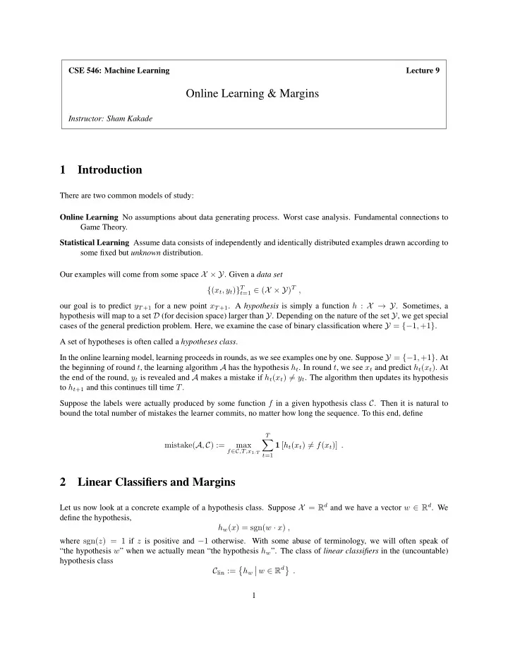
CSE 546: Machine Learning Lecture 9 Online Learning & Margins Instructor: Sham Kakade 1 Introduction There are two common models of study: Online Learning No assumptions about data generating process. Worst case analysis. Fundamental connections to Game Theory. Statistical Learning Assume data consists of independently and identically distributed examples drawn according to some fixed but unknown distribution. Our examples will come from some space X × Y . Given a data set t =1 ∈ ( X × Y ) T , { ( x t , y t ) } T our goal is to predict y T +1 for a new point x T +1 . A hypothesis is simply a function h : X → Y . Sometimes, a hypothesis will map to a set D (for decision space) larger than Y . Depending on the nature of the set Y , we get special cases of the general prediction problem. Here, we examine the case of binary classification where Y = {− 1 , +1 } . A set of hypotheses is often called a hypotheses class . In the online learning model, learning proceeds in rounds, as we see examples one by one. Suppose Y = {− 1 , +1 } . At the beginning of round t , the learning algorithm A has the hypothesis h t . In round t , we see x t and predict h t ( x t ) . At the end of the round, y t is revealed and A makes a mistake if h t ( x t ) � = y t . The algorithm then updates its hypothesis to h t +1 and this continues till time T . Suppose the labels were actually produced by some function f in a given hypothesis class C . Then it is natural to bound the total number of mistakes the learner commits, no matter how long the sequence. To this end, define T � mistake( A , C ) := max 1 [ h t ( x t ) � = f ( x t )] . f ∈C ,T,x 1: T t =1 2 Linear Classifiers and Margins Let us now look at a concrete example of a hypothesis class. Suppose X = R d and we have a vector w ∈ R d . We define the hypothesis, h w ( x ) = sgn( w · x ) , where sgn( z ) = 1 if z is positive and − 1 otherwise. With some abuse of terminology, we will often speak of “the hypothesis w ” when we actually mean “the hypothesis h w ”. The class of linear classifiers in the (uncountable) hypothesis class � w ∈ R d � � � C lin := h w . 1

Note that w and αw yield the same linear classifier for any scalar α > 0 . Suppose we have a data set that is linearly separable . That is, there is a w ∗ such that, ∀ t ∈ [ T ] , y t = sgn( w ∗ · x t ) . (1) Separability means that y t ( w ∗ · x t ) > 0 for all t . The minimum value of this quantity over the data set is referred to as the margin . Let us make the assumption that the margin is lower bounded by 1 . Assumption M. (Margin of 1 ) Without loss of generality suppose � x t � ≤ 1 . Suppose there exists a w ∗ ∈ R d for which (1) holds. Further assume that t ∈ [ T ] y t ( w ∗ · x t ) ≥ 1 , min (2) Note the choice of 1 is arbitrary. Note that the above implies that: 1 t ∈ [ T ] y t ( w ∗ min � w ∗ � · x t ) ≥ � w ∗ � . 2 In other words, the width of the strip separating the positives from the negatives is of size � w ∗ � . Sometimes the margin is define this way (where we assume that instead � w ∗ � = 1 and that the margin is some positive value rather than 1 ). 2.1 The Perceptron Algorithm Algorithm 1 P ERCEPTRON w 1 ← 0 for t = 1 to T do Receive x t ∈ R d Predict sgn( w t · x t ) Receive y t ∈ {− 1 , +1 } if sgn( w t · x t ) � = y t then w t +1 ← w t + y t x t else w t +1 ← w t end if end for The following theorem gives a dimension independent bound on the number of mistakes the P ERCEPTRON algorithm makes. Theorem 2.1. Suppose Assumption M holds. Let T � M T := 1 [sgn( w t · x t ) � = y t ] t =1 denote the number of mistakes the P ERCEPTRON algorithm makes. Then we have, M T ≤ � w ∗ � 2 . Second, if we had instead assumed that � x t � ≤ X + , then the above would be: + � w ∗ � 2 . M T ≤ · X 2 2

Proof. Define m t = 1 if a mistake occurs at time t and 0 otherwise. We have that: w t +1 = w t + m t y t x t Now observe that: � w t +1 − w ∗ � 2 � w t + m t y t x t − w ∗ � 2 = � w t − w ∗ � 2 + 2 m t y t x t ( w t − w ∗ ) + m 2 t y 2 t � x t � 2 = � w t − w ∗ � 2 + 2 m t y t x t ( w t − w ∗ ) + m t � x t � 2 = � w t − w ∗ � 2 + 2 m t y t x t ( w t − w ∗ ) + m t ≤ � w t − w ∗ � 2 − 2 m t + m t ≤ � w t − w ∗ � 2 − m t ≤ where the second to last step holds since we have that: m t y t x t ( w t − w ∗ ) ≤ m t y t x t w t − m t < − m t using the margin assumption and that y t x t w t < 0 when there is a mistake. Hence, we have that: m t ≤ � w t − w ∗ � 2 − � w t +1 − w ∗ � 2 This implies: T m t ≤ � w 1 − w ∗ � 2 − � w T +1 − w ∗ � 2 ≤ � w ∗ � 2 � M T = t =1 which completes the proof. 3 SVMs The SVM loss function can be viewed as a relaxation to the classification loss. The hinge loss on a pair ( x, y ) is defined as: ℓ (( x, y ) , w ) = max { 0 , 1 − yw ⊤ x } In other words, we penalize with a linear loss when yw ⊤ x is 1 or less. Note that we could actually penalize when we have a correct prediction (if 0 ≤ yw ⊤ x ≤ 1 then our prediction is correct and we are still penalized). In this latter case, we call this a ’margin’ mistake. Note that the gradient of this loss is: ∇ ℓ (( x, y ) , w ) = − yx if yw ⊤ x < 1 and the gradient is 0 otherwise. The SVM seeks to minimize the following objective: n 1 � max { 0 , 1 − y i w ⊤ x i } + λ � w � 2 n i =1 As usual, the algorithm can be kernelized. 3