ONE ILL-POSED ESTIMATION PROBLEM OF EXPERIMENTAL PROCESS PARAMETERS. - PowerPoint PPT Presentation

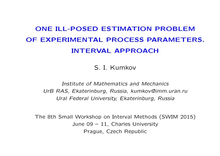
ONE ILL-POSED ESTIMATION PROBLEM OF EXPERIMENTAL PROCESS PARAMETERS. INTERVAL APPROACH S. I. Kumkov Institute of Mathematics and Mechanics UrB RAS, Ekaterinburg, Russia, kumkov@imm.uran.ru Ural Federal University, Ekaterinburg, Russia The 8th Small Workshop on Interval Methods (SWIM 2015) June 09 – 11, Charles University Prague, Czech Republic

The aim of this presentation is to demonstrate one interesting practical problem of estimation of experimental process parameters under uncertainty conditions when components of the parameter vector can be only estimated on the basis of the Interval Analysis approach and available a priori data The work was supported by the RFBR Grant, proj. 15-01-07909. 2

Topics of presentation Experimental process and its model. Measured information and its uncertainty. Interval approach and its peculiarities. Problem formulation and how to solve it ? Computation results. Conclusions. References. 3

Experimental process and its model Description of a reagent activity vs the temperature (similarly to [10,12]) has the form P ( T, a, b, c ) = T 2 a b/c, a > 0 , b > 0 , c > 0 , (1) where T is the temperature (the argument), C ◦ ; P ( · ) is the reagent activity, dimensionless value; a , b , and c are parameters (to be estimated) with dimensions: mole, 1/mole, and (C ◦ ) 2 . 4

Measured information and its uncertainty Results of the experiment are presented as the following collection (a sample with lenght N ) of the reagent activity P measurements: { T n , P n } , n = 2 , N, (2) where values T n are supposed to be know exactly, but the activity values P n are measured with error (noise) P n = P ∗ n + e n , | e n | ≤ e max , n = 2 , N, and for T 1 = 0 , P 1 = 0 , (3) where P n is a noised measurement; P ∗ n is unknown true value under measuring; e n is the error value in the n th measurement; e max is the bound onto the maximal (by modulus) value of the error. By physical reasoning, the conditional exact initial measurement at T 1 = 0 is given zero. 5

Conditions for estimation and a priori information No probabilistic information on errors is known and the sample is dramatically short: N ≈ 5 ∼ 7 measurements only. In (1), parameters a, b and c are merged (“stuck”) that hampers estimation of their own admissible intervals without some additional information. From theoretical estimations and previous experience, the following rough a priori constraints on possible values of the coefficients are given: a ap = [ a ap , a ap ] , b ap = [ b ap , b ap ] , c ap = [ c ap , c ap ] , (4) 0 < a ap < a ap , 0 < b ap < b ap , 0 < c ap < c ap . The LSQM-curve and pointwise estimation of parameters a, b, c and their practically meaningless “cloud-built” intervals are available by only formal application of standard statistical procedures [15–17]. 6

Interval approach and its essence Ideas and methods of the Interval Analysis Theory and Applications arose from the fundamental, pioneer work by L.V. Kantorovich [1]. Nowadays, very effective developments of the theory and computational methods were created by many researchers, e.g . [2–4] and in Russia [5–8]. Special interval algorithms have been elaborated for estimating parameters of experimental chemical processes [9–14]. Remind that essence of this branch of numerical methods theory and application consists in estimation (or identification) of parameters under bounded errors (noises or perturbations) in the input information to be processed, and under complete absence of probabilistic characteristics of errors. 7

The main definitions Uncertainty set (interval) of each measurement (USM). It is the interval of values of measured process consistent with the measurement and the error bound H n = [ h n , h n ] : h n = P n − e max , h n = P n + e max , n = 2 , N, (5) and for n = 1 , H 1 = H (0) = [0] , trivially. Admissible value of the parameter vector and corresponding admissible curve ( a, b, c ) : P ( T n , a, b, c ) ∈ H n , for all n = 1 , N. (6) Informational Set (InfSet) is a totality of admissible values of the parameters vector satisfying the system of interval inequalities (6) { } I ( a, b, c ) = ( a, b, c ) : P ( T n , a, b, c ) ∈ H n , for all n = 1 , N . (7) 8

Measurements and their uncertainty sets (USM) P ,�dim.less true�(model)�values 0.9 noised�measurements _ _ _ _ H uncertainty�intervals n 0.8 2 of�measurements P T�a�b�c ( ,��,��, )�= T a�b c / =�0.1 dim.less , H e 0.7 7 max H 6 0.6 LSQM-curve 0.5 _ _ 0.4 H 5 H 4 0.3 True ( model ) H curve�with _ _ 3 H 0.2 2 a md =�2.0,�mole _ _ _ mole 1 b md =�1/140, 2 (����) 0.1 c md =�100, C _ _ _ _ H T ,�C 1 0 15 25 25 35 45 60 75 If the actual level of errors in the sample is lower the initially given a priori bound e max , the LSQM-curve and values of its parameters could be admissible . 9

Problem formulation Since of very short length of the measurements sample, absence of probabilistic characteristics of the errors, and measurements uncertainty, it is impossible to use (with any good reasoning) the standard statistical methods [15–17]). It is necessary: on the basis of the Interval Analysis methods to built the Informational set I ( a, b, c ) of admissible values (or the Set-membership) of coefficients a , b , and c consistent with the described data. 10

Applied procedures Direct set-estimation approach There are several approaches to solve system (6) of the interval inequalities – classic linear programming methods [1, and many others], – parallelotopes Fiedler M., et al [2], Hansen [3], Jaulin, et al [4], Shary [5], – by the “stripes” method Shary&Sharaya [6], Sharaya [7], Zhilin [8]. More convenient and faster DIRECT method has been elaborated (see, Kumkov and with co-authors [9–14]) that gives exact estimation of the Informational set (7) on part of parameters for each node of the grid on other parameters. In the case under consideration, we represent the { } set I ( a, b, c ) in the form of a collection of its cross-sections I a ( b, c ) for nodes of the grid on the parameter a on its minimal outer interval a ∗ of admissible values. It is performed in contrast, for example, to outer approximation of informational sets in the parallelotope approaches. 11

Three successive auxiliary problems The following auxiliary problems are solved. 1) Introducing the auxiliary merged parameter g = ab/c with g > 0 , its corresponding informational interval g = [ g , g ] is calculated [10,12]. 2) Having the interval equation ad = g , where d = b/c , solve it w.r.t. the auxiliary parameter d as follows: d = g / a ap . As a result in the plane a × d , we obtain the informational set I ( a, d ) with the curve (hyperbolic) lower Fr d ( a ) and upper Fr d ( a ) boundaries as a functions of the parameter a values from its a priori interval a ap . 3) For each value a ∈ a ap we have the interval d ( a ) . So, it becomes possible to construct the informational set I a ( b, c ) of admissible values for parameters b, c for each admissible value of the parameter a . 12

Solution of the auxiliary Problem 1. Informational set of the “merged” parameter g = ab/c _ _ G 4 10 g =�1.43 1,7 _ _ md Partial _ G 4 (��)�= g =�[1.34,�1.59] 10 I g _ _ 1,6 informational _ G ap 4 intervals g =�[0.73,�2.37] 10 1,5 _ _ G 1,4 G 1,3 G 1,2 (��) I g Resultant�informational�interval 2 b ) a ) g ,1/(�����) C ap g _ 4 Admissible�input�data Inadmissible�input�data 10 _ _ 0 0.73 3.13 7.70 2.37 13

Analysis of consistency of a priori data with the measured ones Note that it is worthy to calculate the a priori interval g ap of the parameter g and compare it with the obtained interval g for analysis of consistency of the a priori data (4) on parameters a, b, c with the given sample of measurements (2),(3). 14

Solution of the auxiliary Problem 1. Tube of admissible dependencies true�(model)�values H P ,�dim.less 7 0.9 noised�measurements _ _ _ _ H uncertainty�intervals n 0.8 of�measurements =�0.1 dim.less , e max 2 ( ,��,��, )�= , P T�a�b�c T g g�=�a�b / c 0.7 H Interval�of�admissible�values 0.6 6 of�the�merged�parameter _ 4 0.5 g =�[1.34,�1.59] 10 _ _ _ _ 0.4 H 5 H 4 0.3 Tube H _ _ 3 of�admissible H 0.2 2 dependencies _ _ 0.1 _ _ _ _ H T ,�C 1 0 15 25 25 35 45 60 75 15

Estimating from below the maximal value of the actual error in the sample P ,�dim.less true�(model)�values H * 0.9 7 noised�measurements 2 _ _ P T�a�b�c ( ,��,��, )�= T g , g�=�a�b c / _ _ e 7 { * H uncertainty�intervals n Init 0.8 e =�0.1 dim.less , of�measurements max _ 4 g =�[1.34,�1.59] 10 _ _ 0.7 e =�0.0549 dim.less��~�max{ , | e | } 7 n n The�limit�values: 0.6 e =�0.0457 dim.less , * !!�estimate�from�below max _ 2 4 0.5 g =�1.449 10 ,�1�/�( C ) * _ _ _ ,�1�/�( _ _ 2 H * 4 10 C ) !! g =�1.428 _ _ 6 md 0.4 0.3 H * 4 The�limit _ _ curve�-- “tube” 0.2 H * H * _ _ H * 5 3 2 0.1 _ _ _ _ H T ,�C 1 0 15 25 25 35 45 60 75 16