Multi-parameter regularization for ill-posed problems with noisy - PowerPoint PPT Presentation
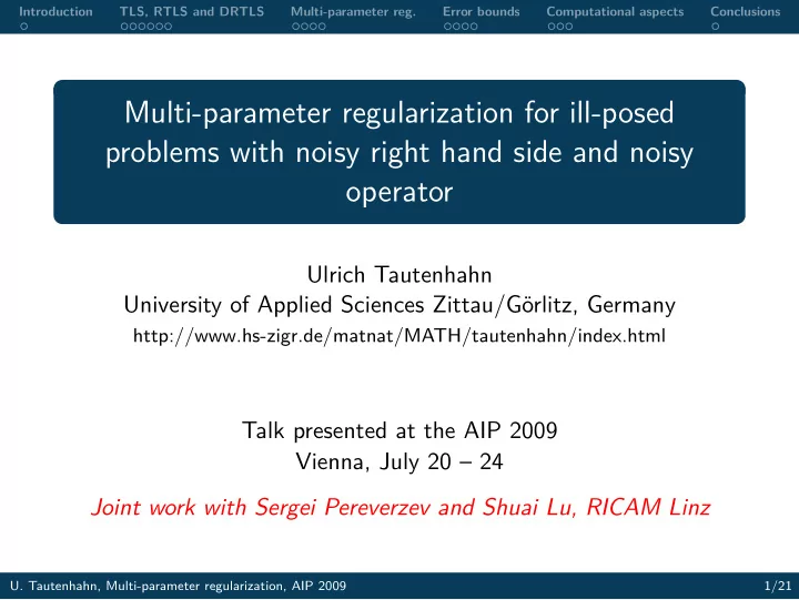
Introduction TLS, RTLS and DRTLS Multi-parameter reg. Error bounds Computational aspects Conclusions Multi-parameter regularization for ill-posed problems with noisy right hand side and noisy operator Ulrich Tautenhahn University of
Introduction TLS, RTLS and DRTLS Multi-parameter reg. Error bounds Computational aspects Conclusions Multi-parameter regularization for ill-posed problems with noisy right hand side and noisy operator Ulrich Tautenhahn University of Applied Sciences Zittau/Görlitz, Germany http://www.hs-zigr.de/matnat/MATH/tautenhahn/index.html Talk presented at the AIP 2009 Vienna, July 20 – 24 Joint work with Sergei Pereverzev and Shuai Lu, RICAM Linz U. Tautenhahn, Multi-parameter regularization, AIP 2009 1/21
Introduction TLS, RTLS and DRTLS Multi-parameter reg. Error bounds Computational aspects Conclusions Content 1 Introduction 2 What is • Total Least Squares (TLS)? • Regularized Total Least Squares (RTLS)? • Dual Regularized Total Least Squares (DRTLS)? 3 What it has to do with multi-parameter regularization? 4 Are there any error bounds for RTLS and DRTLS? 5 How to compute the RTLS and the DRTLS solution? 6 Conclusions U. Tautenhahn, Multi-parameter regularization, AIP 2009 2/21
Introduction TLS, RTLS and DRTLS Multi-parameter reg. Error bounds Computational aspects Conclusions 1 Introduction Problem formulation, notational issues Consider linear ill-conditioned systems x † − unknown (generalized) solution A 0 x = y 0 A 0 ∈ L ( R n , R m ) (generally m ≥ n ) ( A 0 , y 0 ) − error-free data and 1 y δ – given noisy right hand side with � y 0 − y δ � 2 ≤ δ 2 A h – given noisy system matrix with � A 0 − A h � F ≤ h � Ill-conditioning: � y 0 − y δ � 2 ≤ δ �⇒ � x † − x δ,h � 2 ≤ ε � A 0 − A h � F ≤ h U. Tautenhahn, Multi-parameter regularization, AIP 2009 3/21
Introduction TLS, RTLS and DRTLS Multi-parameter reg. Error bounds Computational aspects Conclusions 2 TLS, RTLS and DRTLS Least Squares for A h x ≈ y δ Recall that in the LS problem we solve min x � A h x − y δ � 2 . Alternatively, we look for x, y such that y = A h x : min x,y � y − y δ � 2 subject to y = A h x Total Least Squares for A h x ≈ y δ TLS takes care for perturbations in A h : � A − A h � 2 F + � y − y δ � 2 � � min subject to y = Ax 2 x,y,A Hence, we look for x , y , A to make the system compatible. U. Tautenhahn, Multi-parameter regularization, AIP 2009 4/21
Introduction TLS, RTLS and DRTLS Multi-parameter reg. Error bounds Computational aspects Conclusions How to compute the TLS solution x TLS ? n +1 � v i σ i u T 1 Compute the SVD of ( A h | y δ ) m,n +1 = i i =1 2 Partition U = ( u 1 u 2 ... | u n +1 ) as � U 11 | U 12 � n U = U 21 | U 22 1 3 Then, if U 22 � = 0 , x TLS = − 1 U 12 . U 22 Alternatively, if σ n +1 �∈ σ ( A T h A h ) , x TLS = ( A T h A h − σ n +1 I ) − 1 A T h y δ . U. Tautenhahn, Multi-parameter regularization, AIP 2009 5/21
Introduction TLS, RTLS and DRTLS Multi-parameter reg. Error bounds Computational aspects Conclusions Tikhonov regularization Remember different formulations: � � A h x − y δ � 2 2 + α � Bx � 2 � (i) min 2 x h A h + αB T B A T x = A T � � (ii) h y δ . . . . . . . . . . . . . . . . . . . . . . . . . . . . . . . . . . . . . . . . . . . . . . . . (iii) min x � A h x − y δ � 2 subject to � Bx � 2 ≤ R (iv) min x � Bx � 2 subject to � A h x − y δ � 2 ≤ δ Question: How to introduce TLS in the Tikhonov setting? U. Tautenhahn, Multi-parameter regularization, AIP 2009 6/21
Introduction TLS, RTLS and DRTLS Multi-parameter reg. Error bounds Computational aspects Conclusions Regularized TLS (RTLS) Introduce TLS in the Tikhonov setting (iii) as follows: � A − A h � 2 F + � y − y δ � 2 � � min subject to y = Ax, 2 x,y,A � Bx � 2 ≤ R Dual RTLS Introduce TLS in the Tikhonov setting (iv) as follows: x,y,A � Bx � 2 min subject to y = Ax, 2 � y − y δ � 2 ≤ δ, � A − A h � F ≤ h U. Tautenhahn, Multi-parameter regularization, AIP 2009 7/21
Introduction TLS, RTLS and DRTLS Multi-parameter reg. Error bounds Computational aspects Conclusions Some references on TLS and RTLS Huffel, S. V. and Vanderwalle, J. (1991) The TLS Problem: Computational Aspects and Analysis Philadelphia: SIAM Golub, G. H., Hansen, P. C. and O’Leary, D. P. (1999) Tikhonov regularization and total least squares SIAM J. Matrix Anal. Appl. 21, 185 - 194 Further references on RTLS: Sima, D., Huffel, S. V. and Golub, G. H. (2004), Renaut, R. A. and Guo, H. (2005), Beck, A. and Ben-Tal, A. (2006), Beck, A. and Ben-Tal, A. and Teboulle, M. (2006), Sima, D. (2006), Lu, S. and Pereverzev, S. V. and Tautenhahn, U. (2007), Lampe, J. and Voss, H. (2007,2009) U. Tautenhahn, Multi-parameter regularization, AIP 2009 8/21
Introduction TLS, RTLS and DRTLS Multi-parameter reg. Error bounds Computational aspects Conclusions Some references on DRTLS Lu, S. and Pereverzev, S. V. and Tautenhahn, U. (2007) Regularized total least squares: computational aspects and error bounds RICAM-Preprint 2007-30, SIAM J. Matrix Anal. (accepted) Lu, S. and Pereverzev, S. V. and Tautenhahn, U. (2008) Dual regularized total least squares and multi-parameter regularization Comput. Meth. Appl. Math. 8, 253–262 Lu, S. and Pereverzev, S. V. and Tautenhahn, U. (2008) A model function method in total least squares RICAM-Preprint 2008-18 U. Tautenhahn, Multi-parameter regularization, AIP 2009 9/21
Introduction TLS, RTLS and DRTLS Multi-parameter reg. Error bounds Computational aspects Conclusions 3 RTLS, DRTLS and Multi-parameter regularization? Theorem 1 (RTLS and multi-parameter regularization) Consider the RTLS problem � � A − A h � 2 F + � y − y δ � 2 � min subject to y = Ax, 2 x,y,A � Bx � 2 ≤ R. If the constraint is active, then the solution x RTLS = x R α,β can be obtained by multi-parameter regularization � A h x − y δ � 2 2 + α � Bx � 2 2 + β � x � 2 2 → min where ( α, β ) obey � y δ − A h x R α,β � 2 2 � Bx R α,β � 2 = R and β = − . 1 + � x R α,β � 2 2 U. Tautenhahn, Multi-parameter regularization, AIP 2009 10/21
Introduction TLS, RTLS and DRTLS Multi-parameter reg. Error bounds Computational aspects Conclusions Properties in the general case B � = I Let x = x RTLS be given by h A h + αB T B + βI ) x = A T ( A T h y δ Depending on the choice of R , the solutions are related by R α β solutions R < � Bx T LS � 2 x RT LS � = x T LS α > 0 β < 0 , ∂β/∂R > 0 β = − σ 2 R ≥ � Bx T LS � 2 x RT LS = x T LS α = 0 n +1 • No equivalent interpretation with Tikhonov setting (iii) • Multi-parameter regularization with β < 0 • De-regularization due to the negativity of β U. Tautenhahn, Multi-parameter regularization, AIP 2009 11/21
Introduction TLS, RTLS and DRTLS Multi-parameter reg. Error bounds Computational aspects Conclusions Theorem 2 (DRTLS and multi-parameter regularization) Consider the DRTLS problem x,y,A � Bx � 2 min subject to y = Ax, 2 � y − y δ � 2 ≤ δ, � A − A h � F ≤ h. If the constraints are active, then the solution x DRTLS = x δ,h α,β can be obtained by multi-parameter regularization � A h x − y δ � 2 2 + α � Bx � 2 2 + β � x � 2 2 → min where the parameters α and β obey hδ β = − h 2 − � A h x δ,h α,β − y δ � 2 = δ + h � x δ,h α,β � 2 and . � x δ,h α,β � 2 U. Tautenhahn, Multi-parameter regularization, AIP 2009 12/21
Introduction TLS, RTLS and DRTLS Multi-parameter reg. Error bounds Computational aspects Conclusions Ideas of proof 1 Use classical Lagrange multiplier formulation: L ( x, A, µ, ν ) = � Bx � 2 2 + µ ( � Ax − y δ � 2 2 − δ 2 )+ ν ( � A − A h � 2 F − h 2 ) 2 Optimality conditions: 2 B T Bx + 2 µA T ( Ax − y δ ) = 0 L x = 2 µ ( Ax − y δ ) x T + 2 ν ( A − A h ) = 0 L A = 2 − δ 2 = 0 � Ax − y δ � 2 L µ = F − h 2 = 0 � A − A h � 2 L ν = 3 Manipulation of these equations gives h ( A h x − y δ ) x T A = A h − � ( A h x − y δ ) x T � F 4 Further manipulation gives our characterization result U. Tautenhahn, Multi-parameter regularization, AIP 2009 13/21
Introduction TLS, RTLS and DRTLS Multi-parameter reg. Error bounds Computational aspects Conclusions 6 Error bounds • A 0 ∈ L ( X, Y ) with non-closed range R ( A 0 ) • X, Y – Hilbert spaces • B – strictly pos. self-adjoint (unbounded) operator in X Assumption A1 (Link condition between A 0 and B − 1 ) m � B − a x � ≤ � A 0 x � for some a > 0 , m > 0 Assumption A2 (Solution smoothness) x † ∈ M B,E = x ∈ X : � B p x � ≤ E � � for some p > 0 U. Tautenhahn, Multi-parameter regularization, AIP 2009 14/21
Introduction TLS, RTLS and DRTLS Multi-parameter reg. Error bounds Computational aspects Conclusions Theorem 1 (Order optimality for the RTLS solution) A 1 , A 2 p � � ⇒ � x RTLS − x † � = O p ∈ [1 , 2 + a ] ( δ + h ) p + a R = � Bx † � Extensions: • More general link conditions • More general conditions for solution smoothness • Case 0 < p < 1 ? Problem: Exact magnitude of � Bx † � necessary! U. Tautenhahn, Multi-parameter regularization, AIP 2009 15/21
Recommend
More recommend
Explore More Topics
Stay informed with curated content and fresh updates.
