Numerical approaches to parameter estimates in stochastic evolution - PowerPoint PPT Presentation
/2 Numerical approaches to parameter estimates in stochastic evolution equations driven by fractional Brownian motion Ing. Jan Posp sil, Ph.D. Programs and Algorithms of Numerical Mathematics 13, Prague, May 28 - 31, 2006 1/34
/2 Numerical approaches to parameter estimates in stochastic evolution equations driven by fractional Brownian motion Ing. Jan Posp´ ıˇ sil, Ph.D. Programs and Algorithms of Numerical Mathematics 13, Prague, May 28 - 31, 2006 1/34
Motivation Numerical approaches to parameter estimates in stochastic evolution equations driven by fractional Brownian motion • Mathematical modelling of nanotechnological processes of creating thin films of materials – – possible further research • Analysis of models based on stochastic partial differential equations driven by fractional Brownian motion – parameter estimates – general framework: equations in Hilbert spaces Programs and Algorithms of Numerical Mathematics 13, Prague, May 28 - 31, 2006 2/34
Outline Numerical approaches to parameter estimates in stochastic evolution equations driven by fractional Brownian motion • Stochastic equations in Hilbert spaces • Parameter estimates – estimates based on ergodicity – estimates based on exact variations • Numerical simulations – Linear SDE – Parabolic SPDE Programs and Algorithms of Numerical Mathematics 13, Prague, May 28 - 31, 2006 3/34
Stochastic evolution equations driven by fractional Brownian motion Programs and Algorithms of Numerical Mathematics 13, Prague, May 28 - 31, 2006 4/34
Stochastic equations in Hilbert spaces Numerical approaches to parameter estimates in stochastic evolution equations driven by fractional Brownian motion We consider the linear equation dX ( t ) = AX ( t ) dt + Φ dB H ( t ) , (1) X (0) = x 0 , where ( B H ( t ) , t ≥ 0) is a standard U -valued cylindrical fractional Brownian motion with Hurst parameter H ∈ [1 / 2 , 1) and U is a separable Hilbert space, A : Dom( A ) → V , Dom( A ) ⊂ V , A is the infinitesimal generator of a strongly continuous semigroup ( S ( t ) , t ≥ 0) on the separable Hilbert space V , Φ ∈ L ( U , V ) and x 0 ∈ V is in general random. Programs and Algorithms of Numerical Mathematics 13, Prague, May 28 - 31, 2006 5/34
Solution Numerical approaches to parameter estimates in stochastic evolution equations driven by fractional Brownian motion A solution ( X x 0 ( t ) , t ≥ 0) is considered in the mild form, i.e. for all t ∈ [0 , T ] � t X x 0 ( t ) = S ( t ) x 0 + S ( t − r )Φ dB H ( r ) . (2) 0 [20] T. E. Duncan, B. Maslowski, and B. Pasik-Duncan, Fractional Brownian motion and stochastic equations in Hilbert spaces , Stoch. Dyn. 2 (2002), no. 2, 225–250. • if there is a T 0 > 0 such that � T 0 � T 0 | S ( r )Φ | L 2 ( U , V ) | S ( s )Φ | L 2 ( U , V ) φ ( r − s ) dr ds < ∞ , 0 0 (A1) then the solution exists as a V -valued process • if the semigroup is exponentially stable then there exists a Gaussian centred limiting measure µ ∞ for the solution Programs and Algorithms of Numerical Mathematics 13, Prague, May 28 - 31, 2006 6/34
Strictly stationary solution Numerical approaches to parameter estimates in stochastic evolution equations driven by fractional Brownian motion A measurable V -valued process ( X ( t ) , t ≥ 0) is said to be strictly stationary, if for all k ∈ N and for all arbitrary positive numbers t 1 , t 2 , . . . , t k , the probability distribution of the V k -valued random variable ( X ( t 1 + r ) , X ( t 2 + r ) , . . . , X ( t k + r )) does not depend on r ≥ 0, i.e. Law( X ( t 1 + r ) , X ( t 2 + r ) , . . . , X ( t k + r )) = Law( X ( t 1 ) , X ( t 2 ) , . . . , X ( t k )) for all t 1 , t 2 , . . . , t k , r ≥ 0 Theorem If (A1) is satisfied and the semigroup ( S ( t ) , t ≥ 0) is exponentially stable, then there exists a strictly stationary solution to (1) , i.e. there exists ˜ x, a random variable on (Ω , F , P ) , such that ( X ˜ x ( t ) , t ≥ 0) is a strictly stationary process with Law( X ˜ x ( t )) = µ ∞ , t ≥ 0 . In particular Law(˜ x ) = µ ∞ . Programs and Algorithms of Numerical Mathematics 13, Prague, May 28 - 31, 2006 7/34
Ergodic theorem for arbitrary solution Numerical approaches to parameter estimates in stochastic evolution equations driven by fractional Brownian motion Theorem Let (A1) be satisfied and let ( X x 0 ( t ) , t ≥ 0) be a solution to (1) with initial condition X (0) = x 0 ∈ V , generally random. Let ϕ : R → R be a real function satisfying the following local Lipschitz condition: let there exists a real constant K > 0 and an integer m > 1 such that | ϕ ( x ) − ϕ ( y ) | ≤ K | x − y | (1 + | x | m + | y | m ) (3) for all x , y ∈ R . Let z ∈ Dom( A ∗ ) be arbitrary. Then � T 1 � � X x 0 ( t ) , z � � � � � lim ϕ dt = ϕ � y , z � µ ∞ ( dy ) , a.s.- P . T T →∞ 0 V (4) for all x 0 ∈ V . Programs and Algorithms of Numerical Mathematics 13, Prague, May 28 - 31, 2006 8/34
Parameter estimates Programs and Algorithms of Numerical Mathematics 13, Prague, May 28 - 31, 2006 9/34
Parameter estimates: main results Numerical approaches to parameter estimates in stochastic evolution equations driven by fractional Brownian motion • Parameter estimates based on exact variations – possible from one path observation on a finite interval – suitable for diffusion estimates – applicable also for drift estimates in one-dimensional equation with space-time white noise • Parameter estimates based on ergodicity – consistent results only for T → ∞ – suitable for drift estimates Programs and Algorithms of Numerical Mathematics 13, Prague, May 28 - 31, 2006 10/34
Parameters estimates based on ergodicity Numerical approaches to parameter estimates in stochastic evolution equations driven by fractional Brownian motion Consider the linear equation dX ( t ) = α AX ( t ) dt + Φ dB H ( t ) , (5) X (0) = x 0 , where α > 0 is a real constant parameter. Obviously the operator α A is the infinitesimal generator of the semigroup ( S ( α t ) , t ≥ 0) that is also exponentially stable and there is a limiting measure µ α ∞ = N (0 , Q α ∞ ), where � ∞ � ∞ Q α S ( α u ) QS ∗ ( α v ) φ ( u − v ) du dv ∞ = 0 0 � ∞ � ∞ � u = 1 α − v � S ( u ) QS ∗ ( v ) φ du dv α 2 α 0 0 � ∞ � ∞ = 1 1 1 S ( u ) QS ∗ ( v ) φ ( u − v ) du dv = α 2 H Q 1 ∞ . α 2 α 2 H − 2 0 0 Programs and Algorithms of Numerical Mathematics 13, Prague, May 28 - 31, 2006 11/34
Parameters estimates based on ergodicity Numerical approaches to parameter estimates in stochastic evolution equations driven by fractional Brownian motion Theorem Let (A1) be satisfied and let ( X x 0 ( t ) , t ≥ 0) be a V -valued solution to (5) . Let z ∈ Dom( A ∗ ) be arbitrary and let the limiting measure µ ∞ exists with covariance Q ∞ such that � Q ∞ z , z � V > 0 . Define � 1 � 2 H � Q ∞ z , z � V α T := ˆ . (6) � T 0 | � X x 0 ( t ) , z � V | 2 dt 1 T Then T →∞ ˆ lim α T = α, a.s.- P , for all x 0 ∈ V . Programs and Algorithms of Numerical Mathematics 13, Prague, May 28 - 31, 2006 12/34
Parameters estimates based on ergodicity Numerical approaches to parameter estimates in stochastic evolution equations driven by fractional Brownian motion Theorem Let (A1) be satisfied and let ( X x 0 ( t ) , t ≥ 0) be a V -valued solution to (5) with initial condition x 0 ∈ V such that E | x 0 | 2 V < ∞ . Let the limiting measure µ ∞ exists with covariance Q ∞ such that Tr Q ∞ � = 0 . Define � 1 � 2 H Tr Q ∞ α T := ˆ . (7) � T 1 0 | X x 0 ( t ) | 2 V dt T E Then T →∞ ˆ lim α T = α. Programs and Algorithms of Numerical Mathematics 13, Prague, May 28 - 31, 2006 13/34
Parameters estimates based on variations Numerical approaches to parameter estimates in stochastic evolution equations driven by fractional Brownian motion Theorem Let ( X x 0 ( t ) , t ≥ 0) be a V -valued solution to (1) . Fix 0 < T 1 < T 2 . Define, for j = 0 , 1 , . . . , n, a time grid by t j = T 1 + j δ , where δ = 1 n ( T 2 − T 1 ) . Let z ∈ Dom( A ∗ ) be arbitrary. Then the following limit holds in mean square for all x 0 ∈ V n � |� X x 0 ( t i +1 ) , z � V − � X x 0 ( t i ) , z � V | 1 / H lim n →∞ i =0 = c H [ � Qz , z � V ] 1 / (2 H ) ( T 2 − T 1 ) , (8) where c H = 2 1 / (2 H ) � H +1 � √ π Γ . (9) 2 H Programs and Algorithms of Numerical Mathematics 13, Prague, May 28 - 31, 2006 14/34
Parameters estimates based on variations Numerical approaches to parameter estimates in stochastic evolution equations driven by fractional Brownian motion In particular, if we denote by n 1 |� X x 0 ( t i +1 ) , z � V − � X x 0 ( t i ) , z � V | 1 / H , ˆ � f n ( z ) := c H ( T 2 − T 1 ) i =0 then f n ( z ) − [ � Qz , z � V ] 1 / (2 H ) � 2 � ˆ lim = 0 . (10) n →∞ E Programs and Algorithms of Numerical Mathematics 13, Prague, May 28 - 31, 2006 15/34
Numerical simulations Programs and Algorithms of Numerical Mathematics 13, Prague, May 28 - 31, 2006 16/34
Recommend
More recommend
Explore More Topics
Stay informed with curated content and fresh updates.
