NOTATION Domestic () interest rate: R; foreign: R $ Spot exchange - PDF document
NOTATION Domestic () interest rate: R; foreign: R $ Spot exchange rate $S per 1 Forward rate $F per 1 Basic forex parity relationships 1. Without forward cover, given E (S)=S e , 1 (1+R) $S e (1+R) }Assume cert- or: }
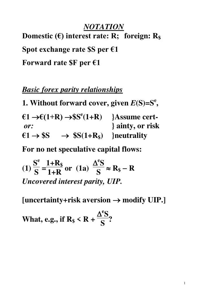
NOTATION Domestic (€) interest rate: R; foreign: R $ Spot exchange rate $S per €1 Forward rate $F per €1 Basic forex parity relationships 1. Without forward cover, given E (S)=S e , €1 €(1+R) $S e (1+R) }Assume cert- or: } ainty, or risk €1 $S $S(1+R $ ) }neutrality For no net speculative capital flows: 1+R or (1a) e S (1) S e S =1+R $ S R $ R Uncovered interest parity, UIP. [uncertainty+risk aversion modify UIP.] What, e.g., if R $ < R + e S S ? 1
2. Using the forward market: €1 €(1+R) $F(1+R) with certainty. Given the equally certain: €1 $S $S(1+R $ ) it's clear that arbitraging implies that: 1+R or (2a) F S S = R $ R (2) F S = 1+R $ 1+R R $ R i.e. ( covered ) interest parity , CIP: fwd premium/discount = interest differential. Q. under CIP, why should hedgers use fwd cover, given that spot transactions can same result? 2
F as a predictor of future S Under certainty , where UIP should hold exactly, S e = S1+R $ 1+R = F, and F (assumed always to satisfy CIP) is the market's expectation of the spot rate. If UIP doesn't hold, an opportunity for profit arises. Assume everything relates to '1 period'. e.g. S e S1+R $ 1+R , then buy €1 for $S borrowed $. After one period, you have accumulated €(1+R), i.e. $S e (1+R), more than you need to repay the debt of $S(1+ R $ ). Given S e , S (and F) rise. Risky world of risk neutrality similar result: UIP gives the rational Exp. of the future spot rate: if you held any other, you'd believe riskless profits available. The rational expectation is that such opportunites have been exploited. Then F is the rational expectation. 3
Risk aversion : UIP contains a risk-premium term: e.g. from the $ perspective, the expected appreciation e S S of the € needs to above the interest differential R $ R for risk-aversion to be overcome and for funds to start to flow into €. Then, F becomes a biased estimate of the future spot rate, even if expectations are rational. Note that bias can also arise because of expectational errors (i.e. non-rational expectations which, unlike RE, will be systematically falsified) i.e. UIP & hence F may indicate the current market expectation (e.g. under risk neutrality) but if expectations are not rational, then F will not be a rational expectation, i.e will be biased ex post . 4
3. Purchasing power parity PPP [P=the goods price- level & Ǐ: E (inflation rate)] Under certainty/risk neutrality, to exclude goods-market arbitrage: PS=P $ : i.e. absolute PPP , unlikely with transactions costs & trade barriers, but we may have relative PPP : At t=0 buy one unit of IR goods priced at P, expected to be worth €P(1+Ǐ) at t=1, or (i) $S e P(1+Ǐ). Alter natively €P=$SP at t=0, so buy $SP/P $ US goods. Expected value for t=1: (ii) $(SP/P $ )P $ (1+Ǐ $ ). To exclude arbitrage, (i)=(ii): $S e (1+Ǐ)=$S(1+Ǐ $ ), or S e /S=(1+Ǐ $ )/(1+Ǐ) which in approx. form is: (3a) e S S Ǐ $ Ǐ 5
Finally using (1a) + (3a): R $ R e S S Ǐ $ Ǐ (4a) R $ Ǐ $ = R Ǐ ' Real interest parity ' (I. Fisher): under UIP and PPP, (expected) real returns should be equated internationally. relevant to Q. of international diversification. Notice that the parity relationships may be put in a slightly different form involving logs: e.g.take logs of (1) S e S =1+R $ 1+R and ln(S e ) ln(S) =s e s= ln(1+R $ ) ln(1+R) R $ R. If S & F were € per $1 (rather than $ per €1) then, in all the parity relationships, swap R & R $ . 6
Siegel’s paradox One reason for writing the relationships in log form is to avoid Siegel’s paradox. If E ($ S )=$ F , then you might think that E (€1/ S )=€1/ F : not so, because the expectation of a function of a random variable is not generally equal to the function of the expectation. In fact when the function is convex, as here, then according to Jensen’s inequality, E (1/ S ) 1/ E ( S ). So if E ( S )= F , then E (1/ S ) 1/ F : i.e. E ( S )= F and E (1/ S )=1/ F can’t both hold. However, if we use E ( log S )= log F , then E ( log 1/ S )= E ( logS )= E(logS )= logF=log1/F. See Baillie and McMahon (1989), p. 166; also Harrison, Michael and Patrick Waldron (2011), Finance , Mathematics for Economics and London: Routledge, p. 356ff. and p. 362ff. 7
OVERSHOOTING foreign & domestic bonds Assume: perfect substitutes, +UIP & short run : sticky goods prices & long run : % P=% M and PPP. A monetary contraction at t=0 (a) Short run : P constant, M P , R (b) Long run : P , so (i) M P & R initial values & (ii) by PPP, S S S(t) R R(t) S 1 R 0 S 0 t=0 t t=0 t (c) Assume rat. exps : S e in SR & LR. R in SR only, during which S overshoots its LR (PPP) value. 8
While R R 0 , depreciation of S after t=0 offsets the additional interest, UIP holding at each t. From UIP, R + e S S =R $ S e is the LR equilibrium value, by rational expectations, and R $ is given. At each step in the SR, R is above its LR value. R rises initially, capital inflows occur, S rises above S e , and the expected depreciation of S offsets the higher R. As P falls, R falls along a path to its original value, and at each stage is accompanied by a lower S, so the expected depreciation is lower. This may be seen alternatively using a version of UIP in log format: s s e =R R $ . 9
The efficient set with exchange-rate risk 2 risky securities, European & US Real returns : Investors IRL US (1) R Ǐ (3) R+x Ǐ $ Securities: € $ (2) R $ x Ǐ (4) R $ Ǐ $ [x e S S ] - asset, E (real return) differs investor - unless PPP, Ǐ $ =Ǐ+x, (1)=(3), (2)=(4) - O/W suppose Ǐ $ =Ǐ+x+e, e random with E (e)=0 & payoff is (1) R Ǐ (3) R Ǐ e (2) R $ Ǐ $ +e (4) R $ Ǐ $ Then a given asset has: *Same E (Real return) investors *More risk for foreign investor. 10
E (Real return) 100% in US IRL investor US investor 100% in IRL Intuition (& calculus) suggests that if the US asset becomes riskier from an IRL perspective because of increased exchange-rate risk, the IRL investor’s optimal portfolio will involve less of the US asset. An equivalent conclusion applies to the IRL asset/US investor. 11
Possible explanations for home bias: financial & informational frictions -departures from PPP; -institutional barriers, capital controls, etc; -transactions costs & taxes [ but see Tesar & Werner: most investors trade foreign shares more often than domestic: odd, if foreign=excess costs ] Uppal: these are not enough. Other possibilities: -benefits of diversification less than expected? -inefficiency of small stock-markets? -investors diversify via stock in multinationals? (but these are more correlated with other domestic firms, than with foreign) -unfamiliarity of foreign assets? (a 'transaction cost'?) 12
Do investors buy the foreign market portfolio? Kang & Stultz - foreign inv. in Japanese securities: - mainly in large firms: 7% of top size quintile, 1¼% bottom, N=1452 1975-1991; - foreign owned averages 3.8% (equally weighted), 6.4% (value weighted); - i.e. not the Japanese market PF; - foreign PF has =5.4%, v. 4.8% for J. market PF.; - foreign PF has no extra return. Product market frictions Obstfeld & Rogoff: start by considering the 'traded ' v. 'non traded' classification of goods. (T, NT) Significance: equity claims on either type of firm can be traded, but earnings must be redeemed in traded goods. - so hold a globally diversified PF, but stock in "NT" industries is all held domestically. 13
- i.e. home bias: domestic investors hold all the "NT" stock, & international diversification only applies to the rest of their PFs. Doesn't explain observed biases. For O&R: goods occupy a place in the continuum: Traded v. Non-traded (v. dichotomy). Trade-costs explicity modelled, model that predicts high & realistic level of home bias. Baxter & Jermann: to hedge human capital risk need short position in domestic traded assets, i.e. % of foreign equity should be higher. Heathcote & Perri: returns to domestic equity covary negatively with labour income, so domestic equity is a good hedge v. labour income risk: 'the international diversification puzzle is not as bad as you think'. Lane & Milesi-Ferretti (2008) [Our] most striking result is that bilateral equity investment is strongly correlated with the underlying pattern of trade in goods. Informational linkages, such as a common language, are also important. 14
Recommend
More recommend
Explore More Topics
Stay informed with curated content and fresh updates.
