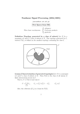
Nonlinear Signal Processing (2004-2005) Course Overview Instituto - PowerPoint PPT Presentation

✬ ✩ Nonlinear Signal Processing (2004-2005) Course Overview Instituto Superior T´ ecnico, Lisbon, Portugal Jo˜ ao Xavier { jxavier } @isr.ist.utl.pt ✫ ✪

✬ ✩ Outline � Motivation : Signal Processing & Related Applications of Differential Geometry ⊲ Optimization ⊲ Kendall’s theory of shapes ⊲ Random Matrix Theory ⋄ Coherent Capacity of Multi-Antenna Systems ⊲ Information Geometry ⊲ Geometrical Interpretation of Jeffreys’ Prior ⊲ Performance Bounds for Constrained or Non-Identifiable Parametric Estimation � Course’s Table of Contents ⊲ Topological manifolds ⊲ Differentiable manifolds ✫ ✪ ⊲ Riemannian manifolds

✬ ✩ Outline � Bibliography ⊲ Recommended textbooks ⊲ Additional material (short notes on specialized topics) � Grading � Discussion, questions, etc ✫ ✪

✬ ✩ Applications of DG: Optimization � Unconstrained minimization problem: x ∗ = arg min x ∈ R n f ( x ) � Iterative line search: given initial point x 0 for k = 0 , 1 , . . . choose descent direction d k solve t ∗ = arg min t ≥ 0 f ( x k + t d k ) x k +1 = x k + t ∗ d k end ✫ ✪

✬ ✩ Applications of DG: Optimization � Sketch: x k +1 d k +1 d k x k x k +2 � � − 1 ∇ f ( x k ) ✫ ✪ ∇ 2 f ( x k ) � Descent direction : d grad = − ∇ f ( x k ) , d newton = −

✬ ✩ Applications of DG: Optimization � Constrained minimization problem: x ∗ = arg h ( x )= 0 f ( x ) min � Iterative line search with projected gradient: given initial point x 0 for k = 0 , 1 , . . . compute d k = Π ( − ∇ f ( x k )) solve t ∗ = arg min t ≥ 0 f ( x k + t d k ) x k +1 = x k + t ∗ d k � x k +1 � 2 return to the constraint surface x k +1 = arg min h ( x )=0 � x − � ✫ ✪ end

✬ ✩ Applications of DG: Optimization � Sketch: − ∇ f ( x k ) x k +1 � x k d k x k +1 h ( x ) = 0 ✫ ✪

✬ ✩ Applications of DG: Optimization � Differential geometry enables a descent algorithm with feasible iterates � Iterative geodesic search: given initial point x 0 for k = 0 , 1 , . . . choose descent direction d k solve t ∗ = arg min t ≥ 0 f ( γ k ( t )) ( γ k ( t ) = geodesic emanating from x k in the direction d k ) x k +1 = γ k ( t ∗ ) end ✫ ✪

✬ ✩ Applications of DG: Optimization � Sketch: d k x k γ k ( t ) x k +1 h ( x ) = 0 � Descent direction : generalizations of d grad and d newton are available � Theory works for abstract spaces (e.g. projective spaces) ✫ ✪

✬ ✩ Applications of DG: Optimization � Example: Signal model y [ t ] = Qx [ t ] + w [ t ] t = 1 , 2 , . . . , T Q : orthogonal matrix ( Q T Q = I N ), x [ t ] : known and w [ t ] iid ∼ N ( 0 , C ) � Maximum-Likelihood Estimate: Q ∗ = arg Q ∈ O ( N ) p ( Y ; Q ) max ⊲ O ( N ) = group of N × N orthogonal matrices ⊲ Y = [ y [1] y [2] · · · y [ T ]] and X = [ x [1] x [2] · · · x [ T ]] ✫ ✪

✬ ✩ Applications of DG: Optimization � Optimization problem: Orthogonal Procrustes rotation Q ∗ Q ∈ O ( N ) � Y − QX � 2 = arg min C − 1 � � � � Q T C − 1 Q � Q T C − 1 � − tr = arg Q ∈ O ( N ) tr min R xx R yx � T � T t =1 y [ t ] x [ t ] T and � ⊲ � R yx = 1 R xx = 1 t =1 x [ t ] x [ t ] T T T � Note: the eigenstructure of C controls the Hessian of the objective κ ( C − 1 ) = λ max ( C − 1 ) λ min ( C − 1 ) condition number of C − 1 ✫ ✪

✬ ✩ Applications of DG: Optimization � Example: N = 5 , T = 100 , C = diag (1 , 1 , 1 , 1 , 1) , κ ( C − 1 ) = 1 2 10 1 10 0 10 −1 10 −2 10 −3 10 0 5 10 15 20 25 30 Iteration ✫ ✪ ◦ =projected gradient � =gradient geodesic descent ⋄ =Newton geodesic descent

✬ ✩ Applications of DG: Optimization � Example: N = 5 , T = 100 , C = diag (0 . 2 , 0 . 4 , 0 . 6 , 0 . 8 , 1) , κ ( C − 1 ) = 5 2 10 1 10 0 10 −1 10 −2 10 −3 10 0 5 10 15 20 25 30 Iteration ✫ ✪ ◦ =projected gradient � =gradient geodesic descent ⋄ =Newton geodesic descent

✬ ✩ Applications of DG: Optimization � Example: N = 5 , T = 100 , C = diag (0 . 02 , 0 . 05 , 0 . 14 , 0 . 37 , 1) , κ ( C − 1 ) = 50 3 10 2 10 1 10 0 10 −1 10 −2 10 0 5 10 15 20 25 30 Iteration ✫ ✪ ◦ =projected gradient � =gradient geodesic descent ⋄ =Newton geodesic descent

✬ ✩ Applications of DG: Optimization � Important: Following geodesics is not necessarily optimal. See: “Optimization algorithms exploiting unitary constraints”, J. Manton, IEEE Trans. on Signal Processing, vol. 50, no. 3, pp. 635–650, March 2002 ✫ ✪

✬ ✩ Applications of DG: Optimization � Bibliography: ⋄ “The geometry of weighted low-rank approximations”, J. Manton et al. , IEEE Trans. on Signal Processing, vol. 51, no. 2, pp. 500–514, February 2003 ⋄ “Efficient algorithms for inferences on Grassmann manifolds”, K. Gallivan et al , Proc. 12 th IEEE Workshop Statistical Signal Processing, 2003 ⋄ “Adaptive eigenvalue computations using Newton’s method on the Grassmann manifold”, E. Lundstrom et al. , SIAM J. Matrix Anal. Appl., vol. 23, no. 3, pp. 819–839, 2002 ⋄ “A Grassmann-Rayleigh quotient iteration for computing invariant subspaces”, P. Absil et al. , SIAM Review, vol. 44, no. 1, pp. 57–73, 2002 ⋄ “Algorithms on the Stiefel manifold for joint diagonalization”, M. Nikpour et al. , IEEE Int. Conf. on Acoust. Speech and Signal Proc. (ICASSP), vol. 2, pp. 1481–1484, 2002 ⋄ “Optimization algorithms exploiting unitary constraints”, J. Manton, IEEE Trans. on Signal Processing, vol. 50, no. 3, pp. 635–650, March 2002 ⋄ “Contravariant adaptation on structured matrix spaces”, T. Moon and J. Gunther, Signal ✫ ✪ Processing, 82, pp. 1389–1410, 2002

✬ ✩ Applications of DG: Optimization � Bibliography (cont.): ⋄ “The geometry of the Newton method on non-compact Lie groups”, R. Mahony and J. Manton, Journal of Global Optimization, vol. 23, pp. 309–327, 2002. ⋄ “Prior knowledge and preferential structures in gradient descent learning algorithms”, R. Mahony and Williamson, Journal of Machine Learning Research, pp. 311–355, 2001. ⋄ “Precoder assisted channel estimation in complex projective space”, J. Manton, IEEE 3 rd Workshop on Sig. Proc. Advanc. on Wir. Comm. (SPAWC), pp. 348–351, 2001 ⋄ “Optimization on Riemannian manifold”, IEEE Proc. 38 th conference on Decision and Control, pp. 888–893, Dec. 1999. ⋄ “Optimum phase-only adaptive nulling”, S. Smith, IEEE Trans. on Signal Processing, vol. 47, no. 7, pp. 1835–1843, July 1999 ⋄ “Motion estimation in computer vision: optimization on Stiefel manifolds”, Y. Ma et al , IEEE Proc. 38 th conference on Decision and Control, vol. 4, pp. 3751–3756, Dec. 1998 ⋄ “The geometry of algorithms with orthogonality constraints”, A. Edelman et al. , SIAM J. ✫ ✪ Matrix Anal. Appl., vol. 20, no. 2, pp. 303–353, 1998

✬ ✩ Applications of DG: Optimization � Bibliography (cont.): ⋄ “Optimal motion from image sequences: a Riemannian viewpoint”, Y. Ma et al , Electronic Research Lab Memorandum, UC Berkeley, 1998 ⋄ “Optimization tecnhiques on Riemannian manifolds”, S. Smith, Fields Institute Communications, vol. 3, pp. 113–136, 1994 ⋄ “Optimization and Dynamical Systems”, U. Helmke and J. Moore, Springer-Verlag, 1994 ⋄ “Geometric optimization methods for adaptive filtering”, S. Smith, PhD Thesis, Harvard University, 1993 ⋄ “Constrained optimization along geodesics”, C. Botsaris, J. Math. Anal. Appl., vol. 79, pp. 295–306, 1981 ✫ ✪

✬ ✩ Applications of DG: Kendall’s theory of shapes Image 1 Image 2 Quotient space [manifold] ⊲ (invariant) shape recognition Database of shapes ⊲ morphing one shape into another ✫ ✪ ⊲ statistics (“mean” shape, clustering)

✬ ✩ Applications of DG: Kendall’s theory of shapes � Bibliography: ⋄ “Multivariate shape analysis”, I. Dryden and K. Mardia, Sankhya: The Indian Journal of Statistics, 55, pp. 460–480, 1993 ⋄ “Procrustes methods in the statistical analysis of shape”, C. Goodall, J. R. Statist. Soc. B, 53, no.2, pp. 285–339, 1991 ⋄ “A survey of the statistical theory of shapes”, D. Kendall, Statist. Sci., 4, pp. pp. 87–120, 1989 ⋄ “Shape manifolds, Procrustean metrics and complex projective spaces”, D. Kendall, Bull. London Math. Soc., 16, pp. 81–121, 1984 ⋄ “Directional Statistics”, K. Mardia and P. Jupp, Wiley Series in Probability and Statistics ✫ ✪

✬ ✩ Applications of DG: Random Matrix Theory � Basic statistics: transformation of random objects in Euclidean spaces ⎧ ⎪ x is a random vector in R n ⎪ ⎪ ⎪ ⎪ ⎨ y ∼ p Y ( y ) = p X ( F − 1 ( y )) J ( y ) x ∼ p X ( x ) ⇒ 1 F : R n → R n smooth, bijective ⎪ J ( y ) = ⎪ det( DF ( F − 1 ( y ))) ⎪ ⎪ ⎪ ⎩ y = F ( x ) p X p Y F R n R n ✫ ✪

✬ ✩ Applications of DG: Random Matrix Theory � Generalization: transformation of random objects in manifolds M , N ⎧ ⎪ x is a random point in M ⎪ ⎪ ⎪ ⎪ ⎨ x ∼ Ω X (exterior form) ⇒ y ∼ Ω Y = . . . ⎪ F : M → N smooth, bijective ⎪ ⎪ ⎪ ⎪ ⎩ y = F ( x ) The answer is provided by the calculus of exterior differential forms Ω X Ω Y F ✫ ✪ M N