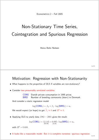
Non-Stationary Time Series and Unit Root Tests Heino Bohn Nielsen - PDF document

Econometrics 2 — Fall 2004 Non-Stationary Time Series and Unit Root Tests Heino Bohn Nielsen 1 of 24 Outline of the Lecture (1) Introduction. (2) Trend stationarity. (3) Unit root processes. (4) Unit root tests. (5) Dickey-Fuller test. (6) Deterministic terms. (7) An alternative test (KPSS). 2 of 24

Introduction • Many economic time series are trending. Important to distinguish between two important cases: (1) A stationary process with a deterministic trend: Shocks have transitory e ff ects. (2) A process with a stochastic trend or a unit root: Shocks have permanent e ff ects. 3 of 24 Trend Stationarity • Consider the stationary AR(1) model with a deterministic linear trend term Y t = θY t − 1 + δ + γt + � t , t = 1 , 2 , ..., T, ( ∗ ) where | θ | < 1 , and Y 0 is an initial value. • The solution for Y t (MA-representation) has the form Y t = θ t Y 0 + µ + µ 1 t + � t + θ� t − 1 + θ 2 � t − 2 + θ 3 � t − 3 + ... The fi rst moments are given by E [ Y t ] = θ t Y 0 + µ + µ 1 t → µ + µ 1 t for T → ∞ , σ 2 V [ Y t ] = 1 − θ 2 . 4 of 24

• The original process, Y t , is not stationary! • The deviation from the mean, y t = Y t − E [ Y t ] = Y t − µ − µ 1 t is a stationary process. The process Y t = y t + µ + µ 1 t is denoted trend-stationary. • Shocks to the process are transitory. We say that the process is mean reverting. Also, we say that the process has an attractor, namely the mean, µ + µ 1 t . 5 of 24 Shock to a Trend Stationarity Process 22.5 20.0 17.5 15.0 12.5 10.0 7.5 5.0 2.5 0.0 0 10 20 30 40 50 60 70 80 90 100 6 of 24

Unit Root Processes • Consider the AR(1) model with a unit root, θ = 1 : Y t = Y t − 1 + δ + � t , t = 1 , 2 , ..., T, ( ∗∗ ) or ∆ Y t = δ + � t , where Y 0 is the initial value. • Note that θ ( L ) = (1 − L ) is not invertible and Y t is non-stationary. • The process ∆ Y t is stationary. We denote Y t a di ff erence stationary process. • If ∆ Y t is stationary while Y t is not, Y t is called integrated of fi rst order, I(1). A process is integrated of order d , I( d ) if ∆ d Y t is stationary while Y t is not. 7 of 24 • The solution for Y t is given by X t X t X t Y t = Y 0 + ∆ Y i = Y 0 + ( δ + � i ) = Y 0 + δt + � i . i =1 i =1 i =1 • The moments are given by E [ Y t ] = Y 0 + δt hX t i = t · σ 2 V [ Y t ] = V i =1 � i Remarks: (1) The e ff ect of the initial value, Y 0 , stays in the process. (2) The innovations, � t , are accumulated to a random walk, P � i . This is the stochastic trend. Shocks have permanent e ff ects. (3) The constant δ is accumulated to a linear trend in Y t . The process in ( ∗∗ ) is denoted a random walk with drift. (4) The process has no attractor. (5) The variance of Y t grows with t . 8 of 24

Shock to a Unit Root Process 50 40 30 20 10 0 10 20 30 40 50 60 70 80 90 100 9 of 24 Why are Unit Roots Important? • Interesting to know if shocks have permanent or transitory e ff ects. Example: If workers ability deteriorates in unemployment, shocks to unemploy- ment could be permanent. This is the hypothesis of hysteresis. • It is important for forecasting to know if the process has an attractor. • The standard distributions for inference in regression models change! Consider the regression model y t = x 0 t β + � t . — If y t and x t are stationary, b β is (asymptotically) normally distributed. — If y t and x t have unit roots, b β is not necessarily normal! Later we look at spurious regression and cointegration. 10 of 24

Unit Root Tests • A good way to think about unit root tests: We compare two relevant models : H 0 and H A . (1) What are the properties of the two models? (2) Do they adequately describe the data? (3) Which one is the null hypothesis? • Consider two alternative test: (1) Dickey-Fuller test: H 0 is a unit root, H A is stationarity. (2) KPSS test: H 0 is stationarity, H A is a unit root. • Often di ffi cult to distinguish in practice (Unit root tests have low power). Many economic time series are persistent, but is the root 0 . 95 or 1 . 0 ? 11 of 24 The Dickey-Fuller (DF) Test • Set up an autoregressive model for y t and test if it has a unit root. Note that MA models are approximated by AR models. • Consider the AR(1) regression model y t = θy t − 1 + � t . The unit root null hypothesis against the stationary alternative corresponds to H 0 : θ = 1 against H A : θ < 1 . • If explosive models are relevant, the alternative could be two-sided: H B : θ 6 = 1 , but rarely seen in practice. 12 of 24

• Alternatively, the model can be formulated as ∆ y t = ( θ − 1) y t − 1 + � t = πy t − 1 + � t , where π = θ − 1 . The hypothesis translates into H 0 : π = 0 against H A : π < 0 . • The Dickey-Fuller (DF) test is simply the t − test of H 0 : b b θ − 1 π b τ = = π ) . se ( b se ( b θ ) The asymptotic distribution of b τ is not normal! The distribution depends on the deterministic components. In the simple case, the 5% critical value is − 1 . 95 and not − 1 . 65 . 13 of 24 Augmented Dickey-Fuller (ADF) test • The DF test is extended to an AR(p) model. Consider an AR(3): y t = θ 1 y t − 1 + θ 2 y t − 2 + θ 3 y t − 3 + � t . It is convenient to rewrite the model as y t − y t − 1 = ( θ 1 − 1) y t − 1 + θ 2 y t − 2 + θ 3 y t − 3 + � t y t − y t − 1 = ( θ 1 − 1) y t − 1 + ( θ 2 + θ 3 ) y t − 2 + θ 3 ( y t − 3 − y t − 2 ) + � t y t − y t − 1 = ( θ 1 + θ 2 + θ 3 − 1) y t − 1 + ( θ 2 + θ 3 )( y t − 2 − y t − 1 ) + θ 3 ( y t − 3 − y t − 2 ) + � t ∆ y t = πY t − 1 + c 1 ∆ y t − 1 + c 2 ∆ y t − 2 + � t , where π = θ 1 + θ 2 + θ 3 − 1 , c 1 = − ( θ 2 + θ 3 ) , and c 2 = − θ 3 . • A unit root in θ ( L ) = 1 − θ 1 L − θ 2 L 2 − θ 3 L 3 corresponds to θ (1) = 0 , i.e. H 0 : π = 0 H A : π < 0 . against The t − test for H 0 is denoted the augmented Dickey-Fuller (ADF) test. 14 of 24

• To determine the number of lags, k , we can use the normal procedures. — General-to-speci fi c testing: Start with k max and delete insigni fi cant lags. — Estimate possible models and use information criteria. • Verbeek suggests to calculate the DF test for all values of k . This is a robustness check, but be careful! Why would we look at tests based on inferior models. • An alternative to the ADF test is to use HAC standard errors for the DF test. Phillips-Perron non-parametric correction for autocorrelation. Likely to be inferior in small samples. 15 of 24 Deterministic Terms in the DF Test • The deterministic speci fi cation is important: — We want an adequate model for the data. — The deterministic speci fi cation changes the asymptotic distribution. • If the variable has a non-zero level, consider a regression model of the form ∆ Y t = πY t − 1 + c 1 ∆ y t − 1 + c 2 ∆ y t − 2 + δ + � t . The ADF test is the t − test, b τ c = b π/ se ( b π ) . The critical value at a 5% level is − 2 . 86 . • If the variable has a deterministic trend, consider a regression model of the form ∆ Y t = πY t − 1 + c 1 ∆ y t − 1 + c 2 ∆ y t − 2 + δ + γt + � t . The ADF test is the t − test, b τ t = b π/ se ( b π ) . The critical value at a 5% level is − 3 . 41 . 16 of 24

The DF Distributions DF with a linear trend, τ t 0.5 DF with a constant, τ c DF, τ 0.4 N(0,1) 0.3 0.2 0.1 -5 -4 -3 -2 -1 0 1 2 3 4 17 of 24 A Note of Caution on Deterministic Terms • The way to think about the inclusion of deterministic terms is via the factor representation: Y t = y t + µ y t = θy t − 1 + � t It follows that ( Y t − µ ) = θ ( Y t − 1 − µ ) + � t Y t = θY t − 1 + (1 − θ ) µ + � t Y t = θY t − 1 + δ + � t which implies a common factor restriction. • If θ = 1 , then implicitly the constant should also be zero, i.e. δ = (1 − θ ) µ = 0 . 18 of 24

• The common factor is not imposed by the normal t − test. Consider Y t = θY t − 1 + δ + � t . The hypotheses H 0 : θ = 1 against H A : θ < 1 , imply H A : Y t = µ + stationary process H 0 : Y t = Y 0 + δt + stochastic trend. • We compare a model with a linear trend against a model with a non-zero level! Potentially di ffi cult to interpret. 19 of 24 • A simple alternative is to consider the combined hypothesis H ∗ 0 : π = δ = 0 . • The hypothesis H ∗ 0 can be tested by running the two regressions H A : ∆ Y t = πY t − 1 + δ + � t H ∗ : ∆ Y t = � t , 0 and perform a likelihood ratio test µ RSS 0 ¶ τ LR = T · log , RSS A where RSS 0 and RSS A denote the residual sum of squares. The 5% critical value is 9.13. 20 of 24