Non-parameteric Estimation of Integral Probability Metrics Bharath - PowerPoint PPT Presentation
Non-parameteric Estimation of Integral Probability Metrics Bharath K. Sriperumbudur , Kenji Fukumizu , Arthur Gretton , , olkopf and Gert R. G. Lanckriet Bernhard Sch The Institute of Statistical Mathematics UC San
Non-parameteric Estimation of Integral Probability Metrics Bharath K. Sriperumbudur ⋆ , Kenji Fukumizu † , Arthur Gretton ‡ , × , olkopf × and Gert R. G. Lanckriet ⋆ Bernhard Sch¨ † The Institute of Statistical Mathematics ⋆ UC San Diego ‡ CMU × MPI for Biological Cybernetics ISIT 2010
Probability Metrics ◮ X : measurable space. ◮ P : set of all probability measures defined on X . ◮ γ : P × P → R + is a notion of distance on P , called the probability metric . Popular example: φ -divergence � � � � d P P ≪ Q X φ d Q , D φ ( P , Q ) := d Q , + ∞ , otherwise where φ : [0 , ∞ ) → ( −∞ , ∞ ] is a convex function. Appropriate choice of φ : Kullback-Leibler divergence, Jensen-Shannon divergence, Total-variation distance, Hellinger distance, χ 2 -distance.
Probability Metrics ◮ X : measurable space. ◮ P : set of all probability measures defined on X . ◮ γ : P × P → R + is a notion of distance on P , called the probability metric . Popular example: φ -divergence � � � � d P P ≪ Q X φ d Q , D φ ( P , Q ) := d Q , + ∞ , otherwise where φ : [0 , ∞ ) → ( −∞ , ∞ ] is a convex function. Appropriate choice of φ : Kullback-Leibler divergence, Jensen-Shannon divergence, Total-variation distance, Hellinger distance, χ 2 -distance.
Applications Two-sample problem: ◮ Given random samples { X 1 , . . . , X m } and { Y 1 , . . . , Y n } drawn i.i.d. from P and Q , respectively. ◮ Determine: are P and Q different?
Applications Two-sample problem: ◮ Given random samples { X 1 , . . . , X m } and { Y 1 , . . . , Y n } drawn i.i.d. from P and Q , respectively. ◮ Determine: are P and Q different? ◮ γ ( P , Q ) : distance metric between P and Q . H 0 : P = Q H 0 : γ ( P , Q ) = 0 ≡ H 1 : P � = Q H 1 : γ ( P , Q ) > 0 ◮ Test: Say H 0 if � γ ( P , Q ) < ε . Otherwise say H 1 .
Applications Two-sample problem: ◮ Given random samples { X 1 , . . . , X m } and { Y 1 , . . . , Y n } drawn i.i.d. from P and Q , respectively. ◮ Determine: are P and Q different? ◮ γ ( P , Q ) : distance metric between P and Q . H 0 : P = Q H 0 : γ ( P , Q ) = 0 ≡ H 1 : P � = Q H 1 : γ ( P , Q ) > 0 ◮ Test: Say H 0 if � γ ( P , Q ) < ε . Otherwise say H 1 . Other applications: ◮ Hypothesis testing : Independence test, Goodness of fit test, etc. ◮ Limit theorems (central limit theorem), density estimation, etc.
Estimation of D φ ( P , Q ) ◮ Given random samples { X 1 , . . . , X m } and { Y 1 , . . . , Y n } drawn i.i.d. from P and Q , estimate D φ ( P , Q ). ◮ Well-studied for φ ( t ) = t log t , t ∈ [0 , ∞ ), i.e., Kullback-Liebler divergence. ◮ Approaches: ◮ Histogram estimator based on space partitioning scheme [Wang et al., 2005]. ◮ M-estimation based on the variational characterization [Nguyen et al., 2008], �� � � φ ∗ ( f ) d Q D φ ( P , Q ) = sup f d P − , f : X → R X X where φ ∗ is the convex conjugate of φ .
Estimation of D φ ( P , Q ) ◮ Given random samples { X 1 , . . . , X m } and { Y 1 , . . . , Y n } drawn i.i.d. from P and Q , estimate D φ ( P , Q ). ◮ Well-studied for φ ( t ) = t log t , t ∈ [0 , ∞ ), i.e., Kullback-Liebler divergence. ◮ Approaches: ◮ Histogram estimator based on space partitioning scheme [Wang et al., 2005]. ◮ M-estimation based on the variational characterization [Nguyen et al., 2008], �� � � φ ∗ ( f ) d Q D φ ( P , Q ) = sup f d P − , f : X → R X X where φ ∗ is the convex conjugate of φ .
Estimation of D φ ( P , Q ) ◮ Given random samples { X 1 , . . . , X m } and { Y 1 , . . . , Y n } drawn i.i.d. from P and Q , estimate D φ ( P , Q ). ◮ Well-studied for φ ( t ) = t log t , t ∈ [0 , ∞ ), i.e., Kullback-Liebler divergence. ◮ Approaches: ◮ Histogram estimator based on space partitioning scheme [Wang et al., 2005]. ◮ M-estimation based on the variational characterization [Nguyen et al., 2008], �� � � φ ∗ ( f ) d Q D φ ( P , Q ) = sup f d P − , f : X → R X X where φ ∗ is the convex conjugate of φ .
Estimation of D φ ( P , Q ) ◮ Given random samples { X 1 , . . . , X m } and { Y 1 , . . . , Y n } drawn i.i.d. from P and Q , estimate D φ ( P , Q ). ◮ Well-studied for φ ( t ) = t log t , t ∈ [0 , ∞ ), i.e., Kullback-Liebler divergence. ◮ Approaches: ◮ Histogram estimator based on space partitioning scheme [Wang et al., 2005]. ◮ M-estimation based on the variational characterization [Nguyen et al., 2008], �� � � φ ∗ ( f ) d Q D φ ( P , Q ) = sup f d P − , f : X → R X X where φ ∗ is the convex conjugate of φ .
Properties of Estimators ◮ Computability ◮ Consistency ◮ Rate of convergence Issues: ◮ Though the estimators of D φ ( P , Q ) are consistent, their rate of convergence can be arbitrarily slow depending on P and Q . ◮ Let X ⊂ R d . For large d , the estimator proposed by [Wang et al., 2005] is computationally inefficient.
Properties of Estimators ◮ Computability ◮ Consistency ◮ Rate of convergence Issues: ◮ Though the estimators of D φ ( P , Q ) are consistent, their rate of convergence can be arbitrarily slow depending on P and Q . ◮ Let X ⊂ R d . For large d , the estimator proposed by [Wang et al., 2005] is computationally inefficient.
Integral Probability Metrics ◮ The integral probability metric [M¨ uller, 1997] between P and Q is defined as � � � � � � � � γ F ( P , Q ) = sup f d P − f d Q � . � f ∈ F X X ◮ Many popular probability metrics can be obtained by appropriately choosing F . ◮ Total variation distance : F = � � f : � f � ∞ := sup x ∈ X | f ( x ) | ≤ 1 . � � | f ( x ) − f ( y ) | ◮ Wasserstein distance : F = f : � f � L := sup x � = y ∈ X ≤ 1 . ρ ( x , y ) ◮ Dudley metric : F = { f : � f � L + � f � ∞ ≤ 1 } . ◮ L p metric : F = { f : � f � L p ( X ,µ ) := ( X | f | p d µ ) 1 / p ≤ 1 , 1 ≤ p < ∞} . � ◮ well-studied in probability theory, mass transporation problems, etc.
Outline ◮ Relation between γ F ( P , Q ) and D φ ( P , Q ) ◮ Estimation of γ F ( P , Q ) ◮ Consistency analysis and rate of convergence
γ F ( P , Q ) vs. D φ ( P , Q ) �� � � φ ∗ ( f ) d Q D φ, F ( P , Q ) := sup f d P − f ∈ F X X ◮ D φ, F ( P , Q ) = D φ ( P , Q ) if F is the set of all real-valued measurable functions on X . � 0 , t = 1 ◮ D φ, F ( P , Q ) = γ F ( P , Q ) if φ ( t ) = t � = 1 . + ∞ , ◮ D φ ( P , Q ) = γ F ( P , Q ) if and only if any one of the following hold: � α ( t − 1) , 0 ≤ t ≤ 1 (i) F = { f : � f � ∞ ≤ β − α 2 } and φ ( t ) = for β ( t − 1) , t ≥ 1 some α < β < ∞ . (ii) F = { f : f = c , c ∈ R } , φ ( t ) = α ( t − 1) , t ≥ 0 , α ∈ R ◮ Total-variation is the only φ -divergence that is also an integral probability metric.
γ F ( P , Q ) vs. D φ ( P , Q ) �� � � φ ∗ ( f ) d Q D φ, F ( P , Q ) := sup f d P − f ∈ F X X ◮ D φ, F ( P , Q ) = D φ ( P , Q ) if F is the set of all real-valued measurable functions on X . � 0 , t = 1 ◮ D φ, F ( P , Q ) = γ F ( P , Q ) if φ ( t ) = t � = 1 . + ∞ , ◮ D φ ( P , Q ) = γ F ( P , Q ) if and only if any one of the following hold: � α ( t − 1) , 0 ≤ t ≤ 1 (i) F = { f : � f � ∞ ≤ β − α 2 } and φ ( t ) = for β ( t − 1) , t ≥ 1 some α < β < ∞ . (ii) F = { f : f = c , c ∈ R } , φ ( t ) = α ( t − 1) , t ≥ 0 , α ∈ R ◮ Total-variation is the only φ -divergence that is also an integral probability metric.
γ F ( P , Q ) vs. D φ ( P , Q ) �� � � φ ∗ ( f ) d Q D φ, F ( P , Q ) := sup f d P − f ∈ F X X ◮ D φ, F ( P , Q ) = D φ ( P , Q ) if F is the set of all real-valued measurable functions on X . � 0 , t = 1 ◮ D φ, F ( P , Q ) = γ F ( P , Q ) if φ ( t ) = t � = 1 . + ∞ , ◮ D φ ( P , Q ) = γ F ( P , Q ) if and only if any one of the following hold: � α ( t − 1) , 0 ≤ t ≤ 1 (i) F = { f : � f � ∞ ≤ β − α 2 } and φ ( t ) = for β ( t − 1) , t ≥ 1 some α < β < ∞ . (ii) F = { f : f = c , c ∈ R } , φ ( t ) = α ( t − 1) , t ≥ 0 , α ∈ R ◮ Total-variation is the only φ -divergence that is also an integral probability metric.
γ F ( P , Q ) vs. D φ ( P , Q ) �� � � φ ∗ ( f ) d Q D φ, F ( P , Q ) := sup f d P − f ∈ F X X ◮ D φ, F ( P , Q ) = D φ ( P , Q ) if F is the set of all real-valued measurable functions on X . � 0 , t = 1 ◮ D φ, F ( P , Q ) = γ F ( P , Q ) if φ ( t ) = t � = 1 . + ∞ , ◮ D φ ( P , Q ) = γ F ( P , Q ) if and only if any one of the following hold: � α ( t − 1) , 0 ≤ t ≤ 1 (i) F = { f : � f � ∞ ≤ β − α 2 } and φ ( t ) = for β ( t − 1) , t ≥ 1 some α < β < ∞ . (ii) F = { f : f = c , c ∈ R } , φ ( t ) = α ( t − 1) , t ≥ 0 , α ∈ R ◮ Total-variation is the only φ -divergence that is also an integral probability metric.
Outline ◮ Relation between γ F ( P , Q ) and D φ ( P , Q ) ◮ Estimation of γ F ( P , Q ) ◮ Consistency analysis and rate of convergence
Recommend
More recommend
Explore More Topics
Stay informed with curated content and fresh updates.

