NIPS Feature Selection Challenge: Details On Methods Amir Reza - PDF document

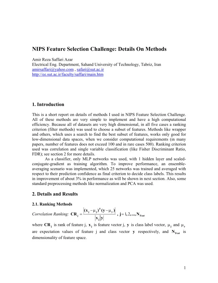
NIPS Feature Selection Challenge: Details On Methods Amir Reza Saffari Azar Electrical Eng. Department, Sahand University of Technology, Tabriz, Iran amirsaffari@yahoo.com , safari@sut.ac.ir http://ee.sut.ac.ir/faculty/saffari/main.htm 1. Introduction This is a short report on details of methods I used in NIPS Feature Selection Challenge. All of these methods are very simple to implement and have a high computational efficiency. Because all of datasets are very high dimensional, in all five cases a ranking criterion (filter methods) was used to choose a subset of features. Methods like wrapper and others, which uses a search to find the best subset of features, works only good for low-dimensional data spaces, when we consider computational requirements (in many papers, number of features does not exceed 100 and in rare cases 500). Ranking criterion used was correlation and single variable classification (like Fisher Discriminant Ratio, FDR); see section 2 for more details. As a classifier, only MLP networks was used, with 1 hidden layer and scaled- conjugate-gradient as training algorithm. To improve performance, an ensemble- averaging scenario was implemented, which 25 networks was trained and averaged with respect to their prediction confidence as final criterion to decide class labels. This results in improvement of about 3% in performance as will be shown in next section. Also, some standard preprocessing methods like normalization and PCA was used. 2. Details and Results 2.1. Ranking Methods − µ T − µ ( x ) ( y ) j j y = = Correlation Ranking: CR , j 1 , 2 , ..., N j Feat x y j µ and µ where CR is rank of feature j, x is feature vector j, y is class label vector, j j j y are expectation values of feature j and class vector y respectively, and N is Feat dimensionality of feature space. 1

µ − µ 2 ( ) j , 1 j , 2 = = FDR Ranking: FDR , j 1 , 2 , ..., N j Feat σ 2 + σ 2 j , 1 j , 2 µ µ where FDR is rank of feature j, and are class mean value of feature vector j for j j , 1 j , 2 σ 2 σ 2 class 1 and 2, respectively, and are class variance value of feature vector j for j , 1 j , 2 class 1 and 2, respectively, and N is dimensionality of feature space. Feat 2.2. Arcene Arcene is a high dimensional dataset with only a few examples, making it difficult to obtain a good generalization. Feature Selection: Features ranked using correlation criteria, those with higher values were selected (about 20%). Preprocessing: Normalized and then applied a linear PCA, those with low contribution to overall variance were removed. Classification: 25 MLP networks with tangent hyperbolic activation functions trained on dataset, those with high value of training performance were selected as a member of committee. Confidence values (outputs) of best networks were averaged to obtain class labels. Results: The best result was 0.1437 on validation set. Individual networks performance was 0.2199 on average, and this shows a 0.0762 improvement using a committee instead of a single network. 2.3. Gisette Gisette is a balanced dataset with respect to number of features and examples, resulting in a good performance. Feature Selection: Features ranked using Fisher’s discriminant criteria, those with higher values were selected (about 10%). Preprocessing: Normalized and then applied a linear PCA, those with low contribution to overall variance were removed. Classification: 25 MLP networks with tangent hyperbolic activation functions trained on dataset, those with high value of training performance were selected as a member of committee. Confidence values (outputs) of best networks were averaged to obtain class labels. 2

Results: The best result was 0.0290 on validation set. Individual networks performance was 0.0309 on average, and this shows very small 0.0019 improvement using a committee instead of a single network, so we can say that only one network is sufficient for this dataset. The main reason is because of higher number of available examples. 2.4. Dexter Dexter is high dimensional dataset with only a few examples, but overall performance is very good with respect to low number of examples. Feature Selection: Features ranked using correlation criteria, those with higher values were selected (about 5%). Preprocessing: None Classification: 25 MLP networks with tangent hyperbolic activation functions, except output which is linear, trained on dataset, those with high value of training performance were selected as a member of committee. Confidence values (outputs) of best networks were averaged to obtain class labels. Results: The best result was 0.0700 on validation set. Individual networks performance was 0.0821 on average, and this shows very small 0.0121 improvement using a committee instead of a single network (not as good as in Arcene). 2.5. Dorothea Dorothea has the highest dimension between datasets, which is also highly biased on negative class. Feature Selection: Features ranked using Fisher’s discriminant criteria, those with higher values were selected (about 1.25%). Preprocessing: Converting all 0 values to –1 in dataset. Classification: 25 MLP networks with tangent hyperbolic activation functions trained on dataset, those with high value of training performance were selected as a member of committee. Confidence values (outputs) of best networks were averaged to obtain class labels. Because of high negative class bias in this dataset, a risk minimization scenario was implemented in class label decision-making. Results: The best result was 0.1020 on validation set. Individual networks performance was 0.1643 on average, and this shows good 0.0623 improvement using a committee instead of a single network. 3

2.6. Madelon Dorothea is the only dataset with a reasonable size of examples and features. Feature Selection: Features ranked using Fisher’s discriminant criteria, those with higher values were selected (about 2%). Preprocessing: Normalization. Classification: 25 MLP networks with tangent hyperbolic activation functions, except output which is linear, trained on dataset, those with high value of training performance were selected as a member of committee. Confidence values (outputs) of best networks were averaged to obtain class labels. Results: The best result was 0.1017 on validation set. Individual networks performance was 0.1309 on average, and this shows very small 0.0292 improvement using a committee instead of a single network (which is not as considerable as in Arcene and Dorothea). 3. Conclusion In this short report on NIPS Feature Selection Challenge, it was shown that some simple feature selection, preprocessing and classification methods could result in a good performance with a very good computational efficiency. On a Pentium IV, 1.8GHz with 256 MB RAM, running a Microsoft Windows 2000 Professional and using MATLAB 6.5 computing rankings of all datasets takes less than 30 minutes. Trainings also finish in less than a 15 min., on average, for all of networks per each dataset (Madelon and Gisette need more computational time than others). It’s obvious that these simple ranking methods are not the best ones to choose a feature subset, but it was shown that could be good candidates when we have computation time constrains. Also it was shown that when we have small training examples, using a committee machine would results in a very good improvement over single classifiers and can statistically obtain a reasonable generalization. The overall performance with these results are shown below and also as Collection2 in workshop website. Balanced Error Area Under Curve Dataset Features Features (%) Train Valid Train Valid arcene 0.0203 0.1437 0.9797 0.8563 2018 20.18 gisette 0.0028 0.0290 0.9972 0.9710 505 10.10 dexter 0.0000 0.0700 1.0000 0.9300 1001 5.00 dorothea 0.0132 0.1020 0.9868 0.8980 1248 1.25 madelon 0.0430 0.1017 0.9570 0.8983 10 2.00 overall 0.0159 0.0893 0.9841 0.9107 7.71 4