New Ideas about Traditional Approach . . . Joint Inversion First - PowerPoint PPT Presentation
Main Objective of Our . . . Gravity . . . Normal Mode . . . New Ideas about Traditional Approach . . . Joint Inversion First Idea: in Brief Details: A Different Basis (as described in a recent A Related Open Problem Second Idea: In Brief
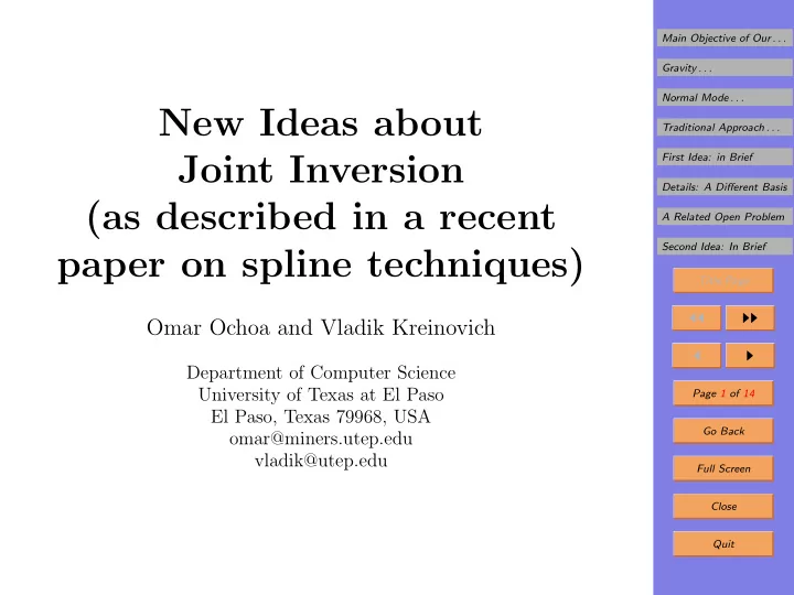
Main Objective of Our . . . Gravity . . . Normal Mode . . . New Ideas about Traditional Approach . . . Joint Inversion First Idea: in Brief Details: A Different Basis (as described in a recent A Related Open Problem Second Idea: In Brief paper on spline techniques) Title Page ◭◭ ◮◮ Omar Ochoa and Vladik Kreinovich ◭ ◮ Department of Computer Science University of Texas at El Paso Page 1 of 14 El Paso, Texas 79968, USA Go Back omar@miners.utep.edu vladik@utep.edu Full Screen Close Quit
Main Objective of Our . . . 1. Main Objective of Our Presentation Gravity . . . • Paper: Paula Berkel, Doreen Fischer, and Volker Michel, Normal Mode . . . “Spline multiresolution and numerical results for joint Traditional Approach . . . gravitation and normal-mode inversion with an out- First Idea: in Brief look on sparse regularisation”, International Journal Details: A Different Basis of Geomathematics , August 2010. A Related Open Problem Second Idea: In Brief • Main objective of the paper: use joint inversion to pro- vide a full 3-D picture of the Earth. Title Page ◭◭ ◮◮ • Geophysically: the authors combine gravity and normal- mode measurements. ◭ ◮ • Our applications: we usually deal with a local geophys- Page 2 of 14 ical analysis. Go Back • Our objective: to describe the main idea that can be Full Screen used in our applications. Close Quit
Main Objective of Our . . . 2. Gravity Measurements: Non-Uniqueness Gravity . . . • Ideally: once we know the gravitational potential field Normal Mode . . . ϕ ( x ), we can determine the density ρ ( x ): Traditional Approach . . . First Idea: in Brief ρ = const · ∇ 2 ϕ ( x ) . Details: A Different Basis A Related Open Problem • In practice: Second Idea: In Brief – we only know the values of ϕ ( x ) with measurement Title Page errors; ◭◭ ◮◮ – we only know the values ϕ ( x ) in some points x – all of which are outside the Earth. ◭ ◮ • Result: we cannot uniquely reconstruct the density Page 3 of 14 ρ ( x ) (“Earth model”) from the gravity measurement Go Back results. Full Screen • Specifically: several different Earth models ρ ( x ) are Close consistent with the same measurement results. Quit
Main Objective of Our . . . 3. Non-Uniqueness (cont-d) Gravity . . . • Additional problem: in the isotropic case, the gravity Normal Mode . . . outside the Earth is ∼ M Traditional Approach . . . R 2 First Idea: in Brief – this is true when the mass is uniformly distributed Details: A Different Basis inside the Earth; A Related Open Problem – this is true when the mass is mostly concentrated Second Idea: In Brief in the center; Title Page – etc. ◭◭ ◮◮ • Conclusion: ◭ ◮ – based on measured gravity values, Page 4 of 14 – we cannot uniquely determine how density is dis- Go Back tributed inside the Earth. Full Screen • Thus, to determine an Earth model, we need to sup- Close plement gravity data with other measurements . Quit
Main Objective of Our . . . 4. Need for Error Bounds and for Faster Computa- Gravity . . . tions Normal Mode . . . • Need for error bounds: Traditional Approach . . . First Idea: in Brief – measurement errors cause errors in the resulting Details: A Different Basis Earth model; A Related Open Problem – it is desirable to find the error bounds on the pa- Second Idea: In Brief rameters of the resulting Earth model. Title Page • Need for faster computations: ◭◭ ◮◮ – in many data processing techniques, we get values on a dense grid; ◭ ◮ – it often turns out that spatial resolution is not so Page 5 of 14 high – especially at depth; Go Back – this means that the difference between ρ ( x ) at two Full Screen neighboring points is not statistically meaningful; – it is desirable to save computation time and only Close generate meaningful values. Quit
Main Objective of Our . . . 5. Normal Mode Measurements Gravity . . . • Gravity measurements provide info about deep layers Normal Mode . . . of Earth. Traditional Approach . . . First Idea: in Brief • To supplement this info, we need to use other geophys- Details: A Different Basis ical info about such deep layers. A Related Open Problem • Such info comes after a strong earthquake, when Second Idea: In Brief – not only a seismic wave reaches a station, Title Page – but also it reaches practically the whole Earth and ◭◭ ◮◮ starts oscillations that go on for some time. ◭ ◮ • Such post-earthquake oscillations are called normal mode Page 6 of 14 oscillations. Go Back • In the paper, gravity measurements are combined with Full Screen the normal mode measurements. Close Quit
Main Objective of Our . . . 6. Traditional Approach to Analyzing Seismic Data Gravity . . . • To understand the new ideas, let us recall the tradi- Normal Mode . . . tional approach. Traditional Approach . . . First Idea: in Brief • First, we reconstruct the velocity (or, equivalently) Details: A Different Basis density model in each 3-D location. A Related Open Problem • The model coming out of the computer program has Second Idea: In Brief some “features”, e.g., areas where: Title Page – either density is higher than around them, ◭◭ ◮◮ – or density is lower than around them. ◭ ◮ • Some of these features are real. Page 7 of 14 • Some are artifacts of the method – caused by uncer- Go Back tainty and incompleteness of data. Full Screen • One of the ways to distinguish between real features Close and artifacts is to use a checkerboard method. Quit
Main Objective of Our . . . 7. Traditional Approach (cont-d) Gravity . . . • Checkerboard method – main idea: Normal Mode . . . Traditional Approach . . . – we add sinusoidal “checkerboard” patterns to the First Idea: in Brief model, Details: A Different Basis – we simulate measurement results corresponding to A Related Open Problem this perturbed model, and Second Idea: In Brief – we apply the algorithm to the simulated measure- Title Page ment results. ◭◭ ◮◮ • Case 1: the algorithm detects the perturbations of this ◭ ◮ spatial size. Page 8 of 14 • Conclusion: features of this size in the original model were real. Go Back • Case 2: the algorithm does not detect perturbations. Full Screen Close • Conclusion: features of this small size are artifacts. Quit
Main Objective of Our . . . 8. First Idea: in Brief Gravity . . . • Problem with the traditional approach: Normal Mode . . . Traditional Approach . . . – we produce a large number of values First Idea: in Brief – and then we, in effect, dismiss many of these values Details: A Different Basis as artifacts. A Related Open Problem • Fact: an arbitrary function can be approximated by Second Idea: In Brief Fourier series Title Page m n � � ρ ( x, y ) = a ij · sin( i · x · ω 0 + j · y · ω 0 + ϕ ) . ◭◭ ◮◮ i =0 j =0 ◭ ◮ • Traditional approach, in effect: find all the values a ij , Page 9 of 14 then dismiss most of them. Go Back • New idea: only find the values a ij that can be (statis- tically reliably) reconstructed. Full Screen • How: we generate a ij one by one until we get too large Close a reconstruction error. Quit
Main Objective of Our . . . 9. Details: A Different Basis Gravity . . . • In general: Normal Mode . . . Traditional Approach . . . – we select a basis e 0 ( x ), e 1 ( x ), etc., and First Idea: in Brief – we represent an arbitrary function f ( x ) as a linear Details: A Different Basis combination of the basis functions e n ( x ): A Related Open Problem ∞ Second Idea: In Brief � f ( x ) = a n · e n ( x ) . Title Page n =0 • Examples of bases: ◭◭ ◮◮ – polynomials 1, x , x 2 , . . . , resulting in Taylor series; ◭ ◮ – sines, resulting in Fourier series. Page 10 of 14 • In the above method: we use sines as the basis. Go Back • In general: other bases are possible. Full Screen • The paper: uses a combination of polynomials and Close sines. Quit
Main Objective of Our . . . 10. A Related Open Problem Gravity . . . • In the proposed method : Normal Mode . . . Traditional Approach . . . – if we cannot recover a ij with a good accuracy, First Idea: in Brief – we stop and dismiss all the values corresponding to Details: A Different Basis this spatial resolution. A Related Open Problem • Problem: this approach does not take into account that Second Idea: In Brief accuracy depends on depth. Title Page • In the checkerboard method: for each spatial frequency, ◭◭ ◮◮ – we keep shallower features if they can be recovered ◭ ◮ from the perturbed data, and Page 11 of 14 – we dismiss deeper features if they cannot be recov- Go Back ered from the perturbed data. Full Screen • Open problem: it is not clear how to do this in the Close proposed method; maybe use wavelets? Quit
Recommend
More recommend
Explore More Topics
Stay informed with curated content and fresh updates.
