Negative velocity fluctuations of pulled reaction fronts Racah - PowerPoint PPT Presentation

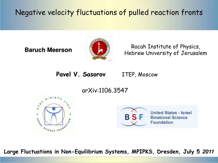
Negative velocity fluctuations of pulled reaction fronts Racah Institute of Physics, Baruch Meerson Hebrew University of Jerusalem Pavel V. Sasorov ITEP, Moscow arXiv:1106.3547 Large Fluctuations in Non-Equilibrium Systems, MPIPKS, Dresden, July 5 2011

• Question: What is the probability that a noisy reaction front moves considerably slower than its deterministic counterpart? For example, can the noise arrest the front motion for some time, or even make it move in the wrong direction?

Outline � Pulled fronts: the deterministic FKPP equation � Stochastic fronts: microscopic model � WKB (large-deviations) formalism: “traveling instantons” and P(c) � Summary and extensions

The FKPP equation Fisher 1937, Kolmogorov, Petrovsky and Piscounov 1937 ∂ = − 2 + ∂ 2 q ( x , t ) q q q ( 1 ) t x A mean-field theory of invasion of an unstable phase, q(x → ∞ , t) = 0, by a stable phase, q(x → −∞ , t) = 1. A fundamental model in mathematical genetics, population biology and chemical kinetics. Also appears in many other fields.

Traveling front solutions (TFSs) : 2 = ξ ξ = − + + − = q ( x , t ) Q ( ), x ct , Q ' ' cQ ' Q Q 0 0 , c 0 , c 0 , c 0 , c 0 , c ≥ c 2 . Legitimate TFSs exist for For a steep initial condition, the solution approaches, at long time, a TFS Q 0,2 ( ξ ) with c=2. This special solution is selected by the dynamics of the leading edge of the front, where Eq. (1) can be linearized around q = 0. The most celebrated example of pulled fronts.

The FKPP equation ignores discreteness of particles and the shot noise. Their impact is dramatic: • Systematic shift of the front velocity δ c~1/ln 2 N (Brunet and Derrida 1997, Brunet, Derrida, Mueller and Munier 2006) • Fluctuations of the front position: D f ~ 1/ln 3 N (Brunet and Derrida 1999,2001; Panja 2003; Brunet, Derrida, Mueller and Munier 2006) N>>1 is the number of particles inside the front region D f only probes typical, relatively small fluctuations of the front position What is the probability P (c) that a noisy front moves, during a long time interval τ , with average velocity c that is considerably smaller than c = 2? This includes the extreme case of c = 0, when the front is standing on average, and even c < 0, when it moves in the wrong direction. But of most interest is the regime of 2-c<<1 when P (c) is not vanishingly small

Microscopic stochastic model: on-site reactions, say A->2A and 2A->A, and random walk on a 1d lattice Evolution of multivariate probability distribution P( n ,t)=P(n 1 ,n 2 ,…,n N ,t) WKB ansatz = − = P ( , t ) exp[ KS ( , t )], / K , n q q n K>>1 is the on-site population size, S( q ,t) is smooth

In the leading order in 1/K one arrives at a Hamilton-Jacobi equation ∂ + ∂ = S H ( , S ) 0 q t q with Hamilton’s function

When random walk is fast this becomes a field theory: a continuous-in-space Hamilton’s mechanics: 1 ∫ = H [ q ( x , t ), p ( x , t )] w dx h [ ] dx 1 ∫ = − ∂ ∂ − ∂ 2 { H ( q , p ) D q p q ( p ) } 0 x x x h H 0 (q,p): on-site Hamilton’s function, h: lattice constant Hamilton’s equations: two coupled PDEs − ∂ = μ λ − μ + ∂ − ∂ ∂ p p 2 q [ ( q ) e ( q ) e ] D [ q 2 ( q p )] t 0 x x x ∂ = − μ λ − + μ − − − ∂ + ∂ p p 2 2 p [ ' ( q )( e 1 ) ' ( q )( e 1 )] D [ p ( p ) ] t 0 x x q(x,t) - rescaled particle concentration – “coordinate”, p(x,t) : “momentum” In context of population extinction risk: Elgart and Kamenev 2004, Meerson and Sasorov 2011

From now on: A->2A, 2A->A in rescaled − p = − + − p 2 H ( q , p ) q ( e 1 ) q ( e 1 ) variables 0 ∂ = − − + ∂ − ∂ ∂ p 2 p 2 q qe q e q 2 ( q p ) t x x x − ∂ = − + − − − ∂ − ∂ p p 2 2 p e 1 2 q ( e 1 ) p ( p ) t x x The “ relaxation trajectories” , q=q (x,t), p=0 are described by the FKPP equation ∂ = − + ∂ 2 2 q ( x , t ) q q q t x Boundary conditions in time: kink-like profiles q(x,0)=q 1 (x), q(x, τ )=q 2 (x) Boundary conditions in space are determined by fixed points of the on-site Hamiltonian: q(- ∞ ,t)=1, p(- ∞ ,t)=0, q(+ ∞ ,t)=0

Calculations simplify in new variables Q=qe -p , P=e p - 1 = − + 2 2 H ( Q , P ) ( Q Q )( P P ) On-site Hamiltonian: 0 = − + Generating function density: F ( q , Q ) q ln( q / Q ) q Q ∂ = − + − + ∂ 2 2 2 Q Q Q 2 QP 2 Q P P ( 1 ) t x ∂ = − − + + − ∂ 2 2 2 P P P 2 QP 2 QP P ( 2 ) t x Boundary conditions: Q(- ∞ ,t)=1; P(- ∞ ,t)=0; Q(+ ∞ ,t)= either 0, or 1 ; P(+ ∞ ,t)=-1 Bernard Derrida observed that Eqs. (1) and (2) also describe the WKB limit of the stochastic FKPP equation ∂ = − + ∂ + ε − η 2 2 Q ( x , t ) Q Q Q Q ( 1 Q ) ( x , t ) t x …, Pechenik and Levine (1999), Doering, Mueller and Smereka (2003), … so most of the following holds for the sFKPP equation too.

Once the Hamilton’s equations are solved, we can calculate the action along the “activation trajectory” q(x,t), p(x,t) and evaluate P (c): ∞ τ P ∫ ∫ − ≈ = ∂ − ln ( c ) K S N dx dt [ p ( x , t ) q ( x , t ) w ] t − ∞ 0 ∞ τ ∫ ∫ = Δ + ∂ − N dx { F dt [ P ( x , t ) Q ( x , t ) W ]} t − ∞ 0 N=Kl d /h>>1 is the number of particles in the front region The model A->2A, 2A->A and random walk has two remarkable symmetries • Let Q 1 (x,t) and P 1 (x,t) be a solution obeying the BCs. Then Q 2 = P 1 (x,-t)+1 and P 2= Q 1 (x,-t) -1 is also a solution with the same BCs. In old variables this is invariance of q(x,t) with respect to time reversal: consequence of detailed balance of underlying microscopic model. • Let Q 1 (x,t) and P 1 (x,t) be a solution obeying the BCs. Then Q 2 = -P 1 (-x,-t) and P 2 =-Q 1 (-x,-t) is also a solution with the same BCs.

Main assumption : at large τ the activation trajectory is described by a Traveling Front Solution (TFS): Q=Q(x-ct), P=P(x-ct) + + − + − = −∞ = ∞ = 2 2 Q ' ' cQ ' Q Q 2 QP 2 Q P 0 , Q ( ) 1 , Q ( ) 0 or 1 − + + 2 − − 2 = −∞ = ∞ = − P ' ' cP ' P P 2 QP 2 QP 0 , P ( ) 0 , P ( ) 1 Find instanton: heteroclinic orbit of the 4 th order dynamical system ξ ξ + = = H [ Q ( ), P ( )] Q ' P ' const 0 Conservation law: 0 reduces the order to 3 rd . Still, for general c the problem appears non-integrable. Numerical solution, however, is straightforward For a TFS P (c) and the action become: ds P − ≈ τ ln ( c ) N , dt ∞ ∞ ∞ ∂ ds H ∫ ∫ ∫ = − ξ + = ξ − = ξ − 2 2 0 d ( cPQ ' W ) d ( P H ) d ( Q Q ) P c ≥ -2 0 ∂ dt P − ∞ − ∞ − ∞ ds ds = + c Follows from detailed balance of microscopic model dt dt − c c

Results Example of numerical fluctuating TFS, c=3/2

Exact solution for c=0: 1 1 = = − Q ( x ) , P ( x ) , + + − x x 1 e 1 e or 1 = = − + x q ( x ) , p ( x ) ln( 1 e ). + x 2 ( 1 e ) As a result, τ ds P = = ≈ − τ , ln ( c 0 ) N / 3 . dt 3

c ≤ -2: equilibrium manifold Q=1, or p=ln q Here the activation trajectory is a time-reversed mean-field TFS with c ≥ 2 ∂ = − − + ∂ 2 2 q ( x , t ) ( q q q ) t x As a result, ds P = = ≈ − τ c , ln ( c 0 ) Nc . dt

Results for the action and ln P (c) ds/dt=c Including exact results for c=0 and c<-2 ds P − ≅ τ ln ( c ) N , dt What happens when c is close to 2 ?

Perturbation theory for 2-c << 1 C=1.96 Strong separation of Q and P profiles. Joint region where two asymptotes can be matched. Action comes from region where |P|~1 . P ≅ − τ − π − ln ( c ) 0 . 0074 ... N exp( / 2 c ) Strongly non-Gaussian, exponentially small in N, and rapidly falls off as c goes down

Work in progress: Comparison with results of Brunet, Derrida, Mueller, and Munier (2006) Thanks to Bernard Derrida for participating in comparison! π ς τ 2 2 n ! ( n ) κ = cumulants ≥ n 2 3 ln N X: front displacement ∫ − β β = X relative to the G ( ) P ( X ) e dX mean-field front position κ ⎡ Γ + ⎤ ∞ π 2 τ β 2 ' ( 1 ∑ β = β = − β = β γ + n g ( ) ln G ( ) n ( ) ⎢ ⎥ Γ + β 3 n ! ln N ( 1 ) ⎣ ⎦ = n 2 σ + ∞ i 1 ∫ P β + β = X g ( ) β ( X ) e d π 2 i σ − ∞ i We evaluated the integral at X<0 via saddle-point approximation. Two different regions: Gaussian dist. and left tail