10/11/19 New Reading (all students) Genetic Algorithms Later this - PDF document
10/11/19 New Reading (all students) Genetic Algorithms Later this week, we will discuss methods to maintain population diversity Reading: Extinction Events Can Accelerate Evolution, Joel Lehman and Risto Miikkulainen. PLOS| one,
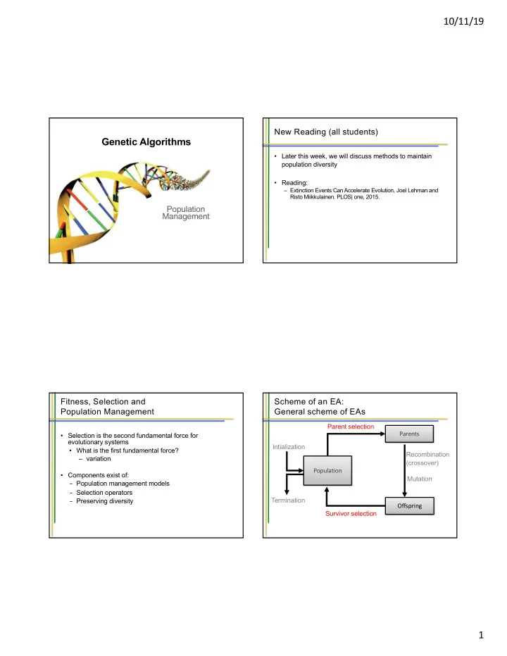
10/11/19 New Reading (all students) Genetic Algorithms • Later this week, we will discuss methods to maintain population diversity • Reading: – Extinction Events Can Accelerate Evolution, Joel Lehman and Risto Miikkulainen. PLOS| one, 2015. Population Management Fitness, Selection and Scheme of an EA: Population Management General scheme of EAs Parent selection Parents • Selection is the second fundamental force for evolutionary systems Intialization • What is the first fundamental force? Recombination – variation (crossover) Population • Components exist of: Mutation - Population management models - Selection operators - Preserving diversity Termination Offspring Survivor selection 1
10/11/19 Population Management Models: Population Management Models: Introduction Fitness based competition • µ -l method: • Selection can occur in two places: – µ: population size – Selection from current generation to take part in mating (parent selection) – l : number of individuals to replace – Selection from parents + offspring to go into next generation • Generational model (survivor selection) • l = µ: all parents replaced by children each generation • Typically, µ children created , though could be more • Selection operators are representation-independent • Steady-state model – They depend on the individual’s fitness (and sometimes • l < µ: some parents remain secondary measures) • l can be as small as 1 • What happens if l is 0? • Generation Gap – The proportion of the population replaced: l /µ Parent Selection: Problem: Fitness-Proportionate Selection Function translation • Probability for individual i to be selected for mating in a population size μ with FPS is: µ ∑ P FPS ( i ) = f i f j j = 1 • Problems include Individual Fitness for Selection Fitness for Sel prob Fitness for Sel prob – Highly fit members can rapidly take over if rest of population is function f Prob for f f + 10 for f + 10 f + 100 for f + 100 much less fit: Premature Convergence A 1 0.1 11 0.275 101 0.326 – At end of runs: fitnesses are similar, loss of selection pressure – Highly susceptible to fitness function translation (shifting) B 4 0.4 14 0.35 104 0.335 • Scaling can fix last two problems C 5 0.5 15 0.375 105 0.339 – Windowing: ! " # = ! # − & ' for generation g Sum 10 1.0 40 1.0 310 1.0 where b is worst fitness in this (last k ) generations – Sigma Scaling: f '( i ) = max( f ( i ) − ( f − c • σ f ),0) where c is a constant, usually 2 2
10/11/19 Definition: Parent Selection: Selection Pressure Rank-based Selection • Attempt to remove problems of FPS by basing selection probabilities on relative rather than absolute fitness • Degree of emphasis on selecting fitter individuals – High selection pressure: higher probability of choosing fitter members • Rank population according to fitness and then base selection probabilities on rank (fittest has rank µ -1 and worst rank 0) – Low selection pressure: lower probability of choosing fitter members • This imposes a sorting overhead on the algorithm, but this is • Formal definition: probability of choosing best member usually negligible compared to the fitness evaluation time over probability of choosing average member. • Ranking schemes not sensitive to fitness function translation • How would you characterize selection pressure = 1? Rank-based Selection: Rank-based selection: Linear Ranking Exponential Ranking • Linear Ranking is limited in selection pressure lin − rank ( i ) = (2 − s ) + 2 i ( s − 1) P µ µ ( µ − 1) , -%. • Parameterised by factor s: 1< s ≤ 2 ! "#$%&'() * = - ∑ 012 , -%0 – measures advantage of best individual • Denominator normalizes probabilities to ensure the sum • Simple 3 member example is 1.0 - , -%0 = , - − 1 Individual Fitness for Rank Sel prob Sel prob Sel prob • Note: 3 function f FPS LR (s = 2) LR (s = 1.5) , − 1 012 A 1 0 0.1 0.0 0.167 "#$%&'() * = , − 1 , - − 1, -%. , B 4 1 0.4 0.33 0.33 • So: ! * ∈ {1, …, :} C 5 2 0.5 0.67 0.5 Sum 10 1.0 1.0 1.0 • , closer to 1 yields lower exponentiality 0 < , < 1 3
10/11/19 Rank-based selection: Parent Selection: Exponential Ranking Tournament Selection • All methods above rely on global population statistics Individual Rank Sel prob Sel prob Sel prob Sel prob Sel prob – Could be a bottleneck esp. with very large population or on LR (s = 2) LR (s = 1.5) ER (c = 1/e) ER (c = 0.1) ER (c = 0.8) parallel architecture A 1 0.000816 0.010408 3.314 e-22 9.000 e-50 3.568 e-06 – Relies on presence of external fitness function which might not B 5 0.004082 0.012041 1.809 e-20 9.000 e-46 8.711 e-06 exist: e.g . evolving game players, evolutionary art C 10 0.008163 0.014082 2.685 e-18 9.000 e-41 2.658 e-05 D 20 0.016326 0.018163 5.915 e -14 9.000 e-31 2.476 e-04 • Idea for a procedure using only local fitness information: E 50 0.040816 0.030408 0.63212 0.9 0.200003 – Pick k members uniformly at random then select the best one Sum 1.0 1.0 1.0 1.0 1.0 from these (of all 50) – Repeat to select more individuals Parent Selection: Parent Selection: Tournament Selection Uniform uniform ( i ) = 1 P • Probability of selecting member i will depend on: µ – Rank of i – Size of sample k • Parents are selected by uniform random distribution • higher k increases selection pressure whenever an operator needs one/some • Uniform parent selection is unbiased - every individual has – Whether contestants are picked with replacement the same probability to be selected • Picking without replacement increases selection pressure – Without replacement, least fit k-1 individuals can never win a tournament • When working with extremely large populations, over- – With replacement, even the least fit individual has probability (1/ µ ) k of being selected (all tournament selection can be used. participants are that member) – Population ranked and divided into 2 groups: top x % in one group – k % of parents chosen from top group, remaining from other – Whether fittest contestant always wins (deterministic) or wins with • Typical value for k is 80 probability p (stochastic) 4
10/11/19 Survivor Selection: Survivor Selection Fitness-based replacement • Elitism • Managing the process of reducing the working memory – Always keep at least one copy of the fittest solution so far of the EA from a set of μ parents and λ offspring to a set – Widely used in both population models (GGA, SSGA) of μ individuals forming the next generation • GENITOR: a.k.a. “delete-worst” • The parent selection mechanisms can also be used for – From Whitley’s original Steady-State algorithm (he also used linear ranking for parent selection) selecting survivors – Rapid takeover: use with large populations (slows takeover) • Survivor selection can be divided into two approaches: • Round-robin tournament – Tournament competitors are: P(t): µ parents and P’(t): µ offspring – Age-Based Selection – Pairwise competitions in round-robin format: • Fitness is not taken into account • Each solution x from P(t) È P’(t) is evaluated against q other randomly chosen solutions • In SSGA can implement as “delete-random” (not • For each comparison, a "win" is assigned if x is better than its opponent recommended) or as first-in-first-out (a.k.a. delete-oldest) • The µ solutions with the greatest number of wins are retained for the next generation – Fitness-Based Replacement – Parameter q allows tuning selection pressure – Typically q = 10, but can be as large as µ - 1 Survivor Selection: Selection Pressure – a different view Fitness-based replacement • Takeover time τ * is a measure to quantify selection • ( µ , l )-selection - based on the set of children only ( l > µ ) pressure - choose best µ • The number of generations it takes until the application • ( µ + l )-selection of selection completely fills the population with copies of - based on the set of parents and children the best individual - choose best µ • For ( µ , l )-selection Goldberg and Deb showed: ln λ τ * = • Often ( µ , l )-selection is preferred for: ln( λ / µ ) – Better in leaving local optima – Better in following moving optima • For proportional selection in a GA with , the ! = # • Historically, l » 7 • µ was a good setting. More recently, takeover time is: (about 460 for pop size = 100) # ln # l » 3 • µ is more popular 5
Recommend
More recommend
Explore More Topics
Stay informed with curated content and fresh updates.
