Nearly Optimal Sparse Fourier Transform Haitham Hassanieh Piotr - PowerPoint PPT Presentation
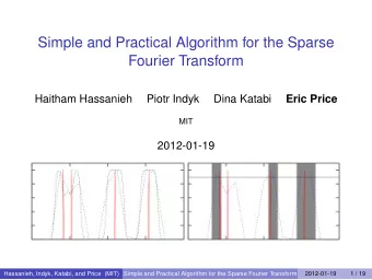
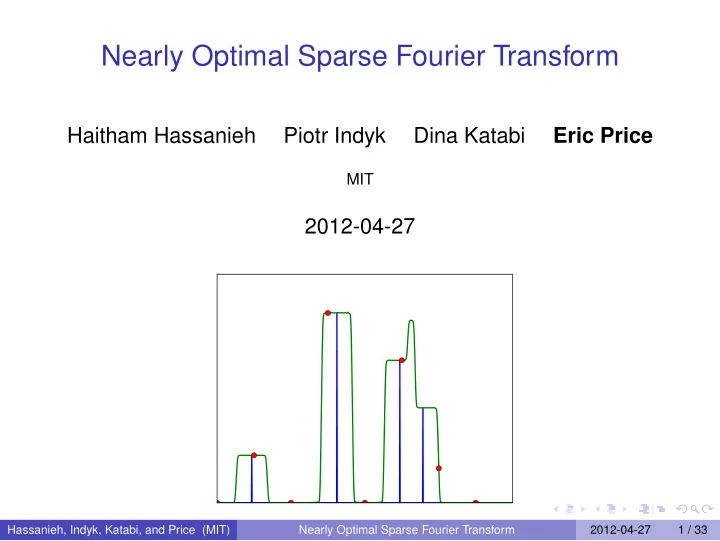
Nearly Optimal Sparse Fourier Transform Haitham Hassanieh Piotr Indyk Dina Katabi Eric Price MIT 2012-04-27 Hassanieh, Indyk, Katabi, and Price (MIT) Nearly Optimal Sparse Fourier Transform 2012-04-27 1 / 33 Outline Introduction 1
Inspiration: arbitrary linear measurements Eppstein-Goodrich ’07 Get linear measurements x i = F − 1 � x of � x i What if we could choose arbitrary linear measurements? Pairwise independent hash: h : [ n ] → [ B ] for B = Θ( k ) . n coordinates B bins For j ∈ [ B ] , observe � � u ′ � i · � u j = x i j = x i h ( i )= j h ( i )= j For each j , set i ∗ = u ′ j / u j and � x ′ i ∗ = u j . Hassanieh, Indyk, Katabi, and Price (MIT) Nearly Optimal Sparse Fourier Transform 2012-04-27 12 / 33
Inspiration: arbitrary linear measurements For j ∈ [ B ] , observe � � u ′ u j = � j = i · � x i x i h ( i )= j h ( i )= j For each j , set i ∗ = u ′ j / u j and � x ′ i ∗ = u j . Hassanieh, Indyk, Katabi, and Price (MIT) Nearly Optimal Sparse Fourier Transform 2012-04-27 13 / 33
Inspiration: arbitrary linear measurements For j ∈ [ B ] , observe � � u ′ u j = � j = i · � x i x i h ( i )= j h ( i )= j For each j , set i ∗ = u ′ j / u j and � x ′ i ∗ = u j . Gives weak sparse recovery: Hassanieh, Indyk, Katabi, and Price (MIT) Nearly Optimal Sparse Fourier Transform 2012-04-27 13 / 33
Inspiration: arbitrary linear measurements For j ∈ [ B ] , observe � � u ′ u j = � j = i · � x i x i h ( i )= j h ( i )= j For each j , set i ∗ = u ′ j / u j and � x ′ i ∗ = u j . Gives weak sparse recovery: ◮ If i alone in bucket h ( i ) , recovered correctly. Hassanieh, Indyk, Katabi, and Price (MIT) Nearly Optimal Sparse Fourier Transform 2012-04-27 13 / 33
Inspiration: arbitrary linear measurements For j ∈ [ B ] , observe � � u ′ u j = � j = i · � x i x i h ( i )= j h ( i )= j For each j , set i ∗ = u ′ j / u j and � x ′ i ∗ = u j . Gives weak sparse recovery: ◮ If i alone in bucket h ( i ) , recovered correctly. ◮ Hence i recovered correctly with 1 − k / B ≥ 15 / 16 probability. Hassanieh, Indyk, Katabi, and Price (MIT) Nearly Optimal Sparse Fourier Transform 2012-04-27 13 / 33
Inspiration: arbitrary linear measurements For j ∈ [ B ] , observe � � u ′ u j = � j = i · � x i x i h ( i )= j h ( i )= j For each j , set i ∗ = u ′ j / u j and � x ′ i ∗ = u j . Gives weak sparse recovery: ◮ If i alone in bucket h ( i ) , recovered correctly. ◮ Hence i recovered correctly with 1 − k / B ≥ 15 / 16 probability. ◮ If i recovered incorrectly, can add one spurious coordinate. Hassanieh, Indyk, Katabi, and Price (MIT) Nearly Optimal Sparse Fourier Transform 2012-04-27 13 / 33
Inspiration: arbitrary linear measurements For j ∈ [ B ] , observe � � u ′ u j = � j = i · � x i x i h ( i )= j h ( i )= j For each j , set i ∗ = u ′ j / u j and � x ′ i ∗ = u j . Gives weak sparse recovery: ◮ If i alone in bucket h ( i ) , recovered correctly. ◮ Hence i recovered correctly with 1 − k / B ≥ 15 / 16 probability. ◮ If i recovered incorrectly, can add one spurious coordinate. ◮ With 3 / 4 probability, less than k / 4 such mistakes. Hassanieh, Indyk, Katabi, and Price (MIT) Nearly Optimal Sparse Fourier Transform 2012-04-27 13 / 33
Inspiration: arbitrary linear measurements For j ∈ [ B ] , observe � � u ′ u j = � j = i · � x i x i h ( i )= j h ( i )= j For each j , set i ∗ = u ′ j / u j and � x ′ i ∗ = u j . Gives weak sparse recovery: ◮ If i alone in bucket h ( i ) , recovered correctly. ◮ Hence i recovered correctly with 1 − k / B ≥ 15 / 16 probability. ◮ If i recovered incorrectly, can add one spurious coordinate. ◮ With 3 / 4 probability, less than k / 4 such mistakes. x ′ is k / 2-sparse. x − � ◮ Hence � Hassanieh, Indyk, Katabi, and Price (MIT) Nearly Optimal Sparse Fourier Transform 2012-04-27 13 / 33
Inspiration: arbitrary linear measurements For j ∈ [ B ] , observe � � u ′ u j = � j = i · � x i x i h ( i )= j h ( i )= j For each j , set i ∗ = u ′ j / u j and � x ′ i ∗ = u j . Gives weak sparse recovery: ◮ If i alone in bucket h ( i ) , recovered correctly. ◮ Hence i recovered correctly with 1 − k / B ≥ 15 / 16 probability. ◮ If i recovered incorrectly, can add one spurious coordinate. ◮ With 3 / 4 probability, less than k / 4 such mistakes. x ′ is k / 2-sparse. x − � ◮ Hence � Goal: construct u , u ′ from Fourier samples. Hassanieh, Indyk, Katabi, and Price (MIT) Nearly Optimal Sparse Fourier Transform 2012-04-27 13 / 33
Inspiration: arbitrary linear measurements For j ∈ [ B ] , observe � � u ′ u j = � j = i · � x i x i h ( i )= j h ( i )= j For each j , set i ∗ = u ′ j / u j and � x ′ i ∗ = u j . Gives weak sparse recovery: ◮ If i alone in bucket h ( i ) , recovered correctly. ◮ Hence i recovered correctly with 1 − k / B ≥ 15 / 16 probability. ◮ If i recovered incorrectly, can add one spurious coordinate. ◮ With 3 / 4 probability, less than k / 4 such mistakes. x ′ is k / 2-sparse. x − � ◮ Hence � Goal: construct u , u ′ from Fourier samples. ◮ Will be able to do this in O ( B log n ) time. Hassanieh, Indyk, Katabi, and Price (MIT) Nearly Optimal Sparse Fourier Transform 2012-04-27 13 / 33
What can you do with Fourier measurements? Time Frequency n -dimensional DFT: O ( n log n ) Hassanieh, Indyk, Katabi, and Price (MIT) Nearly Optimal Sparse Fourier Transform 2012-04-27 14 / 33
What can you do with Fourier measurements? Time Frequency n -dimensional DFT: O ( n log n ) Hassanieh, Indyk, Katabi, and Price (MIT) Nearly Optimal Sparse Fourier Transform 2012-04-27 14 / 33
What can you do with Fourier measurements? Time Frequency n -dimensional DFT: O ( n log n ) n -dimensional DFT of first B terms: O ( n log n ) Hassanieh, Indyk, Katabi, and Price (MIT) Nearly Optimal Sparse Fourier Transform 2012-04-27 14 / 33
What can you do with Fourier measurements? Time Frequency n -dimensional DFT: O ( n log n ) n -dimensional DFT of first B terms: O ( n log n ) B -dimensional DFT of first B terms: O ( B log B ) Hassanieh, Indyk, Katabi, and Price (MIT) Nearly Optimal Sparse Fourier Transform 2012-04-27 14 / 33
What can you do with Fourier measurements? Time Frequency n -dimensional DFT: O ( n log n ) n -dimensional DFT of first B terms: O ( n log n ) B -dimensional DFT of first B terms: O ( B log B ) Hassanieh, Indyk, Katabi, and Price (MIT) Nearly Optimal Sparse Fourier Transform 2012-04-27 14 / 33
Framework “Hashes” into B buckets in B log B time. Analogous to u j = � h ( i )= j � x i . Hassanieh, Indyk, Katabi, and Price (MIT) Nearly Optimal Sparse Fourier Transform 2012-04-27 15 / 33
Framework “Hashes” into B buckets in B log B time. Analogous to u j = � h ( i )= j � x i . Issues: ◮ “Hashing” needs a random hash function ◮ Leakage j = � ◮ Want analog of u ′ h ( i )= j i · � x i . Hassanieh, Indyk, Katabi, and Price (MIT) Nearly Optimal Sparse Fourier Transform 2012-04-27 15 / 33
Framework “Hashes” into B buckets in B log B time. Analogous to u j = � h ( i )= j � x i . Issues: ◮ “Hashing” needs a random hash function ⋆ Access x ′ t = ω − bt x at , so � x ′ at + b = � x t [GMS05] ◮ Leakage j = � ◮ Want analog of u ′ h ( i )= j i · � x i . Hassanieh, Indyk, Katabi, and Price (MIT) Nearly Optimal Sparse Fourier Transform 2012-04-27 15 / 33
Framework “Hashes” into B buckets in B log B time. Analogous to u j = � h ( i )= j � x i . Issues: ◮ “Hashing” needs a random hash function ⋆ Access x ′ t = ω − bt x at , so � x ′ at + b = � x t [GMS05] ◮ Leakage j = � ◮ Want analog of u ′ h ( i )= j i · � x i . ⋆ Time shift x ′ t = x t − 1 : get phase shift � x ′ i = ω i � x i . Hassanieh, Indyk, Katabi, and Price (MIT) Nearly Optimal Sparse Fourier Transform 2012-04-27 15 / 33
Framework “Hashes” into B buckets in B log B time. Analogous to u j = � h ( i )= j � x i . Issues: ◮ “Hashing” needs a random hash function ⋆ Access x ′ t = ω − bt x at , so � x ′ at + b = � x t [GMS05] ◮ Leakage j = � ◮ Want analog of u ′ h ( i )= j i · � x i . ⋆ Time shift x ′ t = x t − 1 : get phase shift � x ′ i = ω i � x i . Hassanieh, Indyk, Katabi, and Price (MIT) Nearly Optimal Sparse Fourier Transform 2012-04-27 15 / 33
Leakage � 1 i < B Let F i = be the “boxcar” filter. (Used in 0 otherwise [GGIMS02,GMS05]) Observe DFT ( F · x , B ) Hassanieh, Indyk, Katabi, and Price (MIT) Nearly Optimal Sparse Fourier Transform 2012-04-27 16 / 33
Leakage � 1 i < B Let F i = be the “boxcar” filter. (Used in 0 otherwise [GGIMS02,GMS05]) Observe DFT ( F · x , B ) = subsample ( DFT ( F · x , n ) , B ) Hassanieh, Indyk, Katabi, and Price (MIT) Nearly Optimal Sparse Fourier Transform 2012-04-27 16 / 33
Leakage � 1 i < B Let F i = be the “boxcar” filter. (Used in 0 otherwise [GGIMS02,GMS05]) Observe DFT ( F · x , B ) = subsample ( DFT ( F · x , n ) , B ) = subsample ( � F ∗ � x , B ) . Hassanieh, Indyk, Katabi, and Price (MIT) Nearly Optimal Sparse Fourier Transform 2012-04-27 16 / 33
Leakage � 1 i < B Let F i = be the “boxcar” filter. (Used in 0 otherwise [GGIMS02,GMS05]) Observe DFT ( F · x , B ) = subsample ( DFT ( F · x , n ) , B ) = subsample ( � F ∗ � x , B ) . DFT � F of boxcar filter is sinc, decays as 1 / i . Hassanieh, Indyk, Katabi, and Price (MIT) Nearly Optimal Sparse Fourier Transform 2012-04-27 16 / 33
Leakage � 1 i < B Let F i = be the “boxcar” filter. (Used in 0 otherwise [GGIMS02,GMS05]) Observe DFT ( F · x , B ) = subsample ( DFT ( F · x , n ) , B ) = subsample ( � F ∗ � x , B ) . DFT � F of boxcar filter is sinc, decays as 1 / i . Need a better filter F ! Hassanieh, Indyk, Katabi, and Price (MIT) Nearly Optimal Sparse Fourier Transform 2012-04-27 16 / 33
Filters Filter (time) Filter (freq) 2.0 25 20 1.5 15 1.0 10 0.5 5 0.0 0 0 20 40 60 80 100 Bin Given | supp ( F ) | = B , concentrate � F . Hassanieh, Indyk, Katabi, and Price (MIT) Nearly Optimal Sparse Fourier Transform 2012-04-27 17 / 33
Filters Filter (time) Filter (freq) 2.0 25 20 1.5 15 1.0 10 0.5 5 0.0 0 0 20 40 60 80 100 Bin Given | supp ( F ) | = B , concentrate � F . Boxcar filter: decays perfectly in time, 1 / t in frequency. ◮ Non-trivial leakage everywhere. Hassanieh, Indyk, Katabi, and Price (MIT) Nearly Optimal Sparse Fourier Transform 2012-04-27 17 / 33
Filters Filter (time) Filter (freq) 1.0 18 16 0.8 14 12 0.6 10 8 0.4 6 4 0.2 2 0.0 0 0 20 40 60 80 100 Bin Given | supp ( F ) | = B , concentrate � F . Boxcar filter: decays perfectly in time, 1 / t in frequency. ◮ Non-trivial leakage everywhere. Gaussians: decay as e − t 2 in time and frequency. � � ◮ Non-trivial leakage to O ( log n · log n ) = O ( log n ) buckets. Hassanieh, Indyk, Katabi, and Price (MIT) Nearly Optimal Sparse Fourier Transform 2012-04-27 17 / 33
Filters Filter (time) Filter (freq) 1.0 80 70 0.8 60 50 0.6 40 0.4 30 20 0.2 10 0.0 0 0 50 100 150 200 Bin Given | supp ( F ) | = B log n , concentrate � F . Boxcar filter: decays perfectly in time, 1 / t in frequency. ◮ Non-trivial leakage everywhere. Gaussians: decay as e − t 2 in time and frequency. � � ◮ Non-trivial leakage to O ( log n · log n ) = O ( log n ) buckets. Still O ( B log n ) time when | supp ( � F ) | = B log n . ◮ Non-trivial leakage to 0 buckets. Hassanieh, Indyk, Katabi, and Price (MIT) Nearly Optimal Sparse Fourier Transform 2012-04-27 17 / 33
Filters Filter (time) Filter (freq) 1.0 80 70 0.8 60 50 0.6 40 0.4 30 20 0.2 10 0.0 0 0 50 100 150 200 Bin Given | supp ( F ) | = B log n , concentrate � F . Boxcar filter: decays perfectly in time, 1 / t in frequency. ◮ Non-trivial leakage everywhere. Gaussians: decay as e − t 2 in time and frequency. � � ◮ Non-trivial leakage to O ( log n · log n ) = O ( log n ) buckets. Still O ( B log n ) time when | supp ( � F ) | = B log n . ◮ Non-trivial leakage to 0 buckets. ◮ Trivial contribution to correct bucket. Hassanieh, Indyk, Katabi, and Price (MIT) Nearly Optimal Sparse Fourier Transform 2012-04-27 17 / 33
Filters Filter (time) Filter (freq) 1.0 80 70 0.8 60 50 0.6 40 0.4 30 20 0.2 10 0.0 0 0 50 100 150 200 Bin � Let G be Gaussian with σ = B log n H be box-car filter of length n / B . Hassanieh, Indyk, Katabi, and Price (MIT) Nearly Optimal Sparse Fourier Transform 2012-04-27 18 / 33
Filters Filter (time) Filter (freq) 0.10 1.2 0.08 1.0 0.06 0.8 0.04 0.6 0.02 0.4 0.00 0.2 0.02 0.0 0 50 100 150 200 Bin � Let G be Gaussian with σ = B log n H be box-car filter of length n / B . Use � F = � G ∗ H . Hassanieh, Indyk, Katabi, and Price (MIT) Nearly Optimal Sparse Fourier Transform 2012-04-27 18 / 33
Filters Filter (time) Filter (freq) 0.10 1.2 0.08 1.0 0.06 0.8 0.04 0.6 0.02 0.4 0.00 0.2 0.02 0.0 0 50 100 150 200 Bin � Let G be Gaussian with σ = B log n H be box-car filter of length n / B . Use � F = � G ∗ H . Hashes correctly to one bucket, leaks to at most 1 bucket. Hassanieh, Indyk, Katabi, and Price (MIT) Nearly Optimal Sparse Fourier Transform 2012-04-27 18 / 33
Filters Filter (time) Filter (freq) 0.10 1.2 0.08 1.0 0.06 0.8 0.04 0.6 0.02 0.4 0.00 0.2 0.02 0.0 0 50 100 150 200 Bin � Let G be Gaussian with σ = B log n H be box-car filter of length n / B . Use � F = � G ∗ H . Hashes correctly to one bucket, leaks to at most 1 bucket. Hassanieh, Indyk, Katabi, and Price (MIT) Nearly Optimal Sparse Fourier Transform 2012-04-27 18 / 33
Properties of filter Filter (frequency): Gaussian * boxcar Hassanieh, Indyk, Katabi, and Price (MIT) Nearly Optimal Sparse Fourier Transform 2012-04-27 19 / 33
Properties of filter Pass region n B “Pass region” of size n / B , outside which is negligible δ . Hassanieh, Indyk, Katabi, and Price (MIT) Nearly Optimal Sparse Fourier Transform 2012-04-27 19 / 33
Properties of filter Super-pass region 9 n 10 B “Pass region” of size n / B , outside which is negligible δ . “Super-pass region”, where ≈ 1. Hassanieh, Indyk, Katabi, and Price (MIT) Nearly Optimal Sparse Fourier Transform 2012-04-27 19 / 33
Properties of filter Bad region “Pass region” of size n / B , outside which is negligible δ . “Super-pass region”, where ≈ 1. Small fraction (say 10%) is “bad region” with intermediate value. Hassanieh, Indyk, Katabi, and Price (MIT) Nearly Optimal Sparse Fourier Transform 2012-04-27 19 / 33
Properties of filter Filter (time): Gaussian · sinc “Pass region” of size n / B , outside which is negligible δ . “Super-pass region”, where ≈ 1. Small fraction (say 10%) is “bad region” with intermediate value. Time domain has support size O ( B log n ) . Hassanieh, Indyk, Katabi, and Price (MIT) Nearly Optimal Sparse Fourier Transform 2012-04-27 19 / 33
Algorithm for exactly sparse signals Original signal x Original signal ˆ x Hassanieh, Indyk, Katabi, and Price (MIT) Nearly Optimal Sparse Fourier Transform 2012-04-27 20 / 33
Algorithm for exactly sparse signals Computed F · x Filtered signal c F ∗ c x Hassanieh, Indyk, Katabi, and Price (MIT) Nearly Optimal Sparse Fourier Transform 2012-04-27 20 / 33
Algorithm for exactly sparse signals F · x aliased to B terms Filtered signal c F ∗ c x Hassanieh, Indyk, Katabi, and Price (MIT) Nearly Optimal Sparse Fourier Transform 2012-04-27 20 / 33
Algorithm for exactly sparse signals F · x aliased to B terms Computed samples of c F ∗ c x Hassanieh, Indyk, Katabi, and Price (MIT) Nearly Optimal Sparse Fourier Transform 2012-04-27 20 / 33
Algorithm for exactly sparse signals F · x aliased to B terms Computed samples of c F ∗ c x Hassanieh, Indyk, Katabi, and Price (MIT) Nearly Optimal Sparse Fourier Transform 2012-04-27 20 / 33
Algorithm for exactly sparse signals F · x aliased to B terms Knowledge about ˆ x Hassanieh, Indyk, Katabi, and Price (MIT) Nearly Optimal Sparse Fourier Transform 2012-04-27 20 / 33
Algorithm for exactly sparse signals F · x aliased to B terms Knowledge about ˆ x Hassanieh, Indyk, Katabi, and Price (MIT) Nearly Optimal Sparse Fourier Transform 2012-04-27 20 / 33
Algorithm for exactly sparse signals F · x aliased to B terms Knowledge about ˆ x Lemma If i is alone in its bucket and in the “super-pass” region, u h ( i ) = � x i . Computing u takes O ( B log n ) time. Hassanieh, Indyk, Katabi, and Price (MIT) Nearly Optimal Sparse Fourier Transform 2012-04-27 20 / 33
Algorithm for perfectly sparse signals Lemma If i is alone in its bucket and in the “super-pass” region, u h ( i ) = � x i . Time-shift x by one and repeat: u ′ x i ω i . h ( i ) = � Divide to find i . Hassanieh, Indyk, Katabi, and Price (MIT) Nearly Optimal Sparse Fourier Transform 2012-04-27 21 / 33
Permutation in time and frequency Can recover coordinates that are alone in their bucket and in the super-pass region. What if coordinates are near each other? Hassanieh, Indyk, Katabi, and Price (MIT) Nearly Optimal Sparse Fourier Transform 2012-04-27 22 / 33
Permutation in time and frequency Can recover coordinates that are alone in their bucket and in the super-pass region. What if coordinates are near each other? Define the “permutation” ( P a , b x ) i = x ai ω − ib . Then � ( P a , b x ) ai + b = � x i . For random a and b , each i is probably “well-hashed.” Hassanieh, Indyk, Katabi, and Price (MIT) Nearly Optimal Sparse Fourier Transform 2012-04-27 22 / 33
Permutation in time and frequency Can recover coordinates that are alone in their bucket and in the super-pass region. What if coordinates are near each other? Define the “permutation” ( P a , b x ) i = x ai ω − ib . Then � ( P a , b x ) ai + b = � x i . For random a and b , each i is probably “well-hashed.” Hassanieh, Indyk, Katabi, and Price (MIT) Nearly Optimal Sparse Fourier Transform 2012-04-27 22 / 33
Overall algorithm Weak sparse recovery: ◮ Permute with random a , b . ◮ Hash to u ◮ Time shift by one, hash to u ′ . ◮ For j ∈ [ B ] ⋆ Choose i ∗ by u ′ j / u j = ω i ∗ . ⋆ Set � x ′ i ∗ = u j . Hassanieh, Indyk, Katabi, and Price (MIT) Nearly Optimal Sparse Fourier Transform 2012-04-27 23 / 33
Overall algorithm Weak sparse recovery: ◮ Permute with random a , b . ◮ Hash to u ◮ Time shift by one, hash to u ′ . ◮ For j ∈ [ B ] ⋆ Choose i ∗ by u ′ j / u j = ω i ∗ . ⋆ Set � x ′ i ∗ = u j . Full sparse recovery: x ′ ← WeakRecovery ( x , k ) ◮ � ◮ k → k / 2, x → ( x − x ′ ) , repeat. Hassanieh, Indyk, Katabi, and Price (MIT) Nearly Optimal Sparse Fourier Transform 2012-04-27 23 / 33
Overall algorithm Weak sparse recovery: ◮ Permute with random a , b . ◮ Hash to u ◮ Time shift by one, hash to u ′ . ◮ For j ∈ [ B ] ⋆ Choose i ∗ by u ′ j / u j = ω i ∗ . ⋆ Set � x ′ i ∗ = u j . Full sparse recovery: x ′ ← WeakRecovery ( x , k ) ◮ � ◮ k → k / 2, x → ( x − x ′ ) , repeat. Time dominated by hash to B r = k / 2 r buckets in round r : ◮ B r log n to hash x . x ′ takes O ( | supp ( � ◮ Hashing � x ′ ) | ) = O ( k ) . Hassanieh, Indyk, Katabi, and Price (MIT) Nearly Optimal Sparse Fourier Transform 2012-04-27 23 / 33
Overall algorithm Weak sparse recovery: ◮ Permute with random a , b . ◮ Hash to u ◮ Time shift by one, hash to u ′ . ◮ For j ∈ [ B ] ⋆ Choose i ∗ by u ′ j / u j = ω i ∗ . ⋆ Set � x ′ i ∗ = u j . Full sparse recovery: x ′ ← WeakRecovery ( x , k ) ◮ � ◮ k → k / 2, x → ( x − x ′ ) , repeat. Time dominated by hash to B r = k / 2 r buckets in round r : ◮ B r log n to hash x . x ′ takes O ( | supp ( � ◮ Hashing � x ′ ) | ) = O ( k ) . Time � ( k 2 r log n + k ) = O ( k log n ) . Hassanieh, Indyk, Katabi, and Price (MIT) Nearly Optimal Sparse Fourier Transform 2012-04-27 23 / 33
Outline Introduction 1 Special case: exactly sparse signals 2 General case: approximately sparse signals 3 Experiments 4 Hassanieh, Indyk, Katabi, and Price (MIT) Nearly Optimal Sparse Fourier Transform 2012-04-27 24 / 33
Nearly sparse signals What happens if only 90 % of the mass lies in top k coordinates, not 100 % ? x i | 2 > � x tail � 2 Want to find most “heavy” coordinates i with | � 2 / k . Hassanieh, Indyk, Katabi, and Price (MIT) Nearly Optimal Sparse Fourier Transform 2012-04-27 25 / 33
Nearly sparse signals What happens if only 90 % of the mass lies in top k coordinates, not 100 % ? x i | 2 > � x tail � 2 Want to find most “heavy” coordinates i with | � 2 / k . Lemma Each i is “well-hashed” with large constant probability over the permutation ( a , b ) . If i is well-hashed, then with time shift c we have x i ω ci + η u h ( i ) = � so that for random c, the noise η is bounded by E [ | η | 2 ] � � x tail � 2 2 / B Hassanieh, Indyk, Katabi, and Price (MIT) Nearly Optimal Sparse Fourier Transform 2012-04-27 25 / 33
Recovering well-hashed i ω ci � x i x i ω c π ( i ) + η with With good probability over c , get u h ( i ) = � | η | < | � x i | / 10. Hassanieh, Indyk, Katabi, and Price (MIT) Nearly Optimal Sparse Fourier Transform 2012-04-27 26 / 33
Recovering well-hashed i ω ci � x i + η x i ω c π ( i ) + η with With good probability over c , get u h ( i ) = � | η | < | � x i | / 10. Hassanieh, Indyk, Katabi, and Price (MIT) Nearly Optimal Sparse Fourier Transform 2012-04-27 26 / 33
Recovering well-hashed i ω ci � x i + η θ x i ω c π ( i ) + η with With good probability over c , get u h ( i ) = � | η | < | � x i | / 10. Phase error | θ | ≤ sin − 1 ( | η | x i | ) < 0 . 11. | � Hassanieh, Indyk, Katabi, and Price (MIT) Nearly Optimal Sparse Fourier Transform 2012-04-27 26 / 33
Recovering well-hashed i ω ci � x i + η θ x i ω c π ( i ) + η with With good probability over c , get u h ( i ) = � | η | < | � x i | / 10. Phase error | θ | ≤ sin − 1 ( | η | x i | ) < 0 . 11. | � True for random c . For a fixed γ , run on c and c + γ to observe ω γπ ( i ) to within 0 . 22. Hassanieh, Indyk, Katabi, and Price (MIT) Nearly Optimal Sparse Fourier Transform 2012-04-27 26 / 33
Recovering well-hashed i ω γ i observation Find i from n / k possibilities in bucket. Choose any γ , then observe ω γ i to within ± 0 . 1 radians. Constant number of bits, so hope for Θ( log ( n / k )) observations. Hassanieh, Indyk, Katabi, and Price (MIT) Nearly Optimal Sparse Fourier Transform 2012-04-27 27 / 33
Recovering well-hashed i ω i We know i to within R . Set γ = ⌊ n / R ⌋ . Restrict and repeat, log ( n / k ) times. Hassanieh, Indyk, Katabi, and Price (MIT) Nearly Optimal Sparse Fourier Transform 2012-04-27 28 / 33
Recovering well-hashed i ω γ i We know i to within R . Set γ = ⌊ n / R ⌋ . Restrict and repeat, log ( n / k ) times. Hassanieh, Indyk, Katabi, and Price (MIT) Nearly Optimal Sparse Fourier Transform 2012-04-27 28 / 33
Recovering well-hashed i observation ω γ i We know i to within R . Set γ = ⌊ n / R ⌋ . Restrict and repeat, log ( n / k ) times. Hassanieh, Indyk, Katabi, and Price (MIT) Nearly Optimal Sparse Fourier Transform 2012-04-27 28 / 33
Recovering well-hashed i observation ω γ i We know i to within R . Set γ = ⌊ n / R ⌋ . Restrict and repeat, log ( n / k ) times. Hassanieh, Indyk, Katabi, and Price (MIT) Nearly Optimal Sparse Fourier Transform 2012-04-27 28 / 33
Recovering well-hashed i ω i We know i to within R . Set γ = ⌊ n / R ⌋ . Restrict and repeat, log ( n / k ) times. Hassanieh, Indyk, Katabi, and Price (MIT) Nearly Optimal Sparse Fourier Transform 2012-04-27 28 / 33
Recovering well-hashed i ω i We know i to within R . Set γ = ⌊ n / R ⌋ . Restrict and repeat, log ( n / k ) times. Hassanieh, Indyk, Katabi, and Price (MIT) Nearly Optimal Sparse Fourier Transform 2012-04-27 28 / 33
Problem: constant failure probability per measurement ω γ i observation We only estimate ω γ i well with 90 % probability. Some of the log ( n / k ) restrictions will go awry. Hassanieh, Indyk, Katabi, and Price (MIT) Nearly Optimal Sparse Fourier Transform 2012-04-27 29 / 33
Problem: constant failure probability per measurement ω γ i We only estimate ω γ i well with 90 % probability. Some of the log ( n / k ) restrictions will go awry. Hassanieh, Indyk, Katabi, and Price (MIT) Nearly Optimal Sparse Fourier Transform 2012-04-27 29 / 33
Recommend
More recommend
Explore More Topics
Stay informed with curated content and fresh updates.
