N 1 N i . (26) i 1 Can bootstrap the standard error. 25 - PowerPoint PPT Presentation
A Course in Applied Econometrics 1 . The Basic Methodology Lecture 11 : Difference - in - Differences Estimation Standard case: outcomes are observed for two groups for two time periods. One of the groups is exposed to a treatment in the second
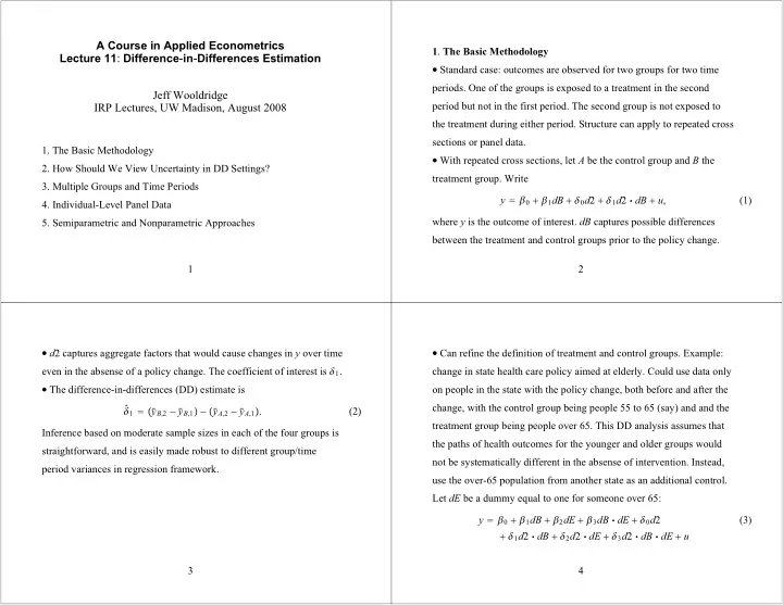
A Course in Applied Econometrics 1 . The Basic Methodology Lecture 11 : Difference - in - Differences Estimation � Standard case: outcomes are observed for two groups for two time periods. One of the groups is exposed to a treatment in the second Jeff Wooldridge period but not in the first period. The second group is not exposed to IRP Lectures, UW Madison, August 2008 the treatment during either period. Structure can apply to repeated cross sections or panel data. 1. The Basic Methodology � With repeated cross sections, let A be the control group and B the 2. How Should We View Uncertainty in DD Settings? treatment group. Write 3. Multiple Groups and Time Periods y � � 0 � � 1 dB � � 0 d 2 � � 1 d 2 � dB � u , (1) 4. Individual-Level Panel Data where y is the outcome of interest. dB captures possible differences 5. Semiparametric and Nonparametric Approaches between the treatment and control groups prior to the policy change. 1 2 � d 2 captures aggregate factors that would cause changes in y over time � Can refine the definition of treatment and control groups. Example: even in the absense of a policy change. The coefficient of interest is � 1 . change in state health care policy aimed at elderly. Could use data only � The difference-in-differences (DD) estimate is on people in the state with the policy change, both before and after the � 1 � � y change, with the control group being people 55 to 65 (say) and and the � � B ,2 � y � B ,1 � � � y � A ,2 � y � A ,1 � . (2) treatment group being people over 65. This DD analysis assumes that Inference based on moderate sample sizes in each of the four groups is the paths of health outcomes for the younger and older groups would straightforward, and is easily made robust to different group/time not be systematically different in the absense of intervention. Instead, period variances in regression framework. use the over-65 population from another state as an additional control. Let dE be a dummy equal to one for someone over 65: y � � 0 � � 1 dB � � 2 dE � � 3 dB � dE � � 0 d 2 (3) � � 1 d 2 � dB � � 2 d 2 � dE � � 3 d 2 � dB � dE � u 3 4
� The OLS estimate � � 3 is 2 . How Should We View Uncertainty in DD Settings ? � Standard approach: all uncertainty in inference enters through � 3 � �� y � � B , E ,2 � y � B , E ,1 � � � y � B , N ,2 � y � B , N ,1 �� (4) � �� y � A , E ,2 � y � A , E ,1 � � � y � A , N ,2 � y � A , N ,1 �� sampling error in estimating the means of each group/time period combination. Long history in analysis of variance. where the A subscript means the state not implementing the policy and � Recently, different approaches have been suggested that focus on the N subscript represents the non-elderly. This is the different kinds of uncertainty – perhaps in addition to sampling error in difference-in-difference-in-differences (DDD) estimate. estimating means. Bertrand, Duflo, and Mullainathan (2004), Donald � Can add covariates to either the DD or DDD analysis to (hopefully) and Lang (2007), Hansen (2007a,b), and Abadie, Diamond, and control for compositional changes. � Can use multiple time periods and groups. Hainmueller (2007) argue for additional sources of uncertainty. � In fact, in the “new” view, the additional uncertainty is often assumed to swamp the sampling error in estimating group/time period means. 5 6 � One way to view the uncertainty introduced in the DL framework – � Using Kentucky and a total sample size of 5,626, the DD estimate of and a perspective explicitly taken by ADH – is that our analysis should the policy change is about 19.2% (longer time on workers’ compensation) with t � 2.76. Using Michigan, with a total sample size better reflect the uncertainty in the quality of the control groups. � Issue: In the standard DD and DDD cases, the policy effect is just of 1,524, the DD estimate is 19.1% with t � 1.22. (Adding controls identified in the sense that we do not have multiple treatment or control does not help reduce the standard error, nor does it change the point groups assumed to have the same mean responses. So, for example, the estimates.) There seems to be plenty of uncertainty in the estimate even DL approach does not allow inference in such cases. with a pretty large sample size. Should we conclude that we really have � Example from Meyer, Viscusi, and Durbin (1995) on estimating the no usable data for inference? effects of benefit generosity on length of time a worker spends on workers’ compensation. MVD have the standard DD before-after setting. 7 8
� As in cluster sample cases, can write 3 . Multiple Groups and Time Periods � With many time periods and groups, in BDM (2004) and Hansen y igt � � gt � z igt � gt � u igt , i � 1,..., M gt ; (6 ) (2007b) is useful. At the individual level, a model at the individual level where intercepts and slopes are allowed y igt � � t � � g � x gt � � z igt � gt � v gt � u igt , (5) to differ across all � g , t � pairs. Then, we think of � gt as i � 1,..., M gt , � gt � � t � � g � x gt � � v gt . (7) where i indexes individual, g indexes group, and t indexes time. Full set Think of (7) as a model at the group/time period level. of time effects, � t , full set of group effects, � g , group/time period � As discussed by BDM, a common way to estimate and perform covariates (policy variabels), x gt , individual-specific covariates, z igt , inference in (5) is to ignore v gt , so the individual-level observations are unobserved group/time effects, v gt , and individual-specific errors, u igt . treated as independent. When v gt is present, the resulting inference can Interested in � . be very misleading. 9 10 � BDM and Hansen (2007b) allow serial correlation in � In any case, proceed as if M gt are large enough to ignore the � gt ; instead, the uncertainty comes through v gt in � v gt : t � 1,2,..., T � but assume independence across g . estimation error in the � � If we view (7) as ultimately of interest, there are simple ways to (7). The minimum distance approach from cluster sample notes proceed. We observe x gt , � t is handled with year dummies,and � g just effectively drops v gt from (7) and views � gt � � t � � g � x gt � as a set of deterministic restrictions to be imposed on � gt . Inference using the represents group dummies. The problem, then, is that we do not � gt . Here, observe � gt . Use OLS on the individual-level data to estimate the � gt , efficient MD estimator uses only sampling variation in the � � u igt � � 0 and the group/time period sizes, M gt , are assuming E � z igt we proceed ignoring estimation error, and so act as if (7) is, for t � 1,..., T , g � 1,..., G , reasonably large. � Sometimes one wishes to impose some homogeneity in the slopes – � gt � � t � � g � x gt � � v gt . � (8) say, � gt � � g or even � gt � � – in which case pooling can be used to impose such restrictions. 11 12
� We can apply the BDM findings and Hansen (2007a) results directly � Hansen (2007b), noting that the OLS estimator (the fixed effects to this equation. Namely, if we estimate (8) by OLS – which means full estimator) applied to (8) is inefficient when v gt is serially uncorrelated, year and group effects, along with x gt – then the OLS estimator has proposes feasible GLS. When T is small, estimating the parameters in � � Var � v g � , where v g is the T � 1error vector for each g , is difficult satisfying properties as G and T both increase, provided � v gt : t � 1,2,..., T � is a weakly dependent time series for all g . The when group effects have been removed. Bias in estimates based on the � gt , disappears as T � � , but can be substantial even for simulations in BDM and Hansen (2007a) indicate that cluster-robust FE residuals, v moderate T . In AR(1) case, � � comes from inference, where each cluster is a set of time periods, work reasonably well when � v gt � follows a stable AR(1) model and G is moderately � gt on v � g , t � 1 , t � 2,..., T , g � 1,..., G . v (9) large. 13 14 � One way to account for bias in � � Even when G and T are both large, so that the unadjusted AR � : use fully robust inference. But, as Hansen (2007b) shows, this can be very inefficient relative to his coefficients also deliver asymptotic efficiency, the bias-adusted � and then use the bias-adjusted suggestion to bias-adjust the estimator � estimates deliver higher-order improvements in the asymptotic estimator in feasible GLS. (Hansen covers the general AR � p � model.) distribution. � Hansen shows that an iterative bias-adjusted procedure has the same � One limitation of Hansen’s results: they assume � x gt : t � 1,..., T � � in the case � � should work well: G and T asymptotic distribution as � are strictly exogenous. If we just use OLS, that is, the usual fixed both tending to infinity. Most importantly for the application to DD effects estimate – strict exogeneity is not required for consistency as T � � . Of course, GLS approaches to serial correlation generally rely problems, the feasible GLS estimator based on the iterative procedure has the same asymptotic distribution as the infeasible GLS etsimator on strict exogeneity. In intervention analyis, might be concerned if the when G � � and T is fixed. policies can switch on and off over time. 15 16
Recommend
More recommend
Explore More Topics
Stay informed with curated content and fresh updates.
