N 1 N 1 IV x i y i s i z i s i z i (2) 3. Imputation i 1 - PowerPoint PPT Presentation

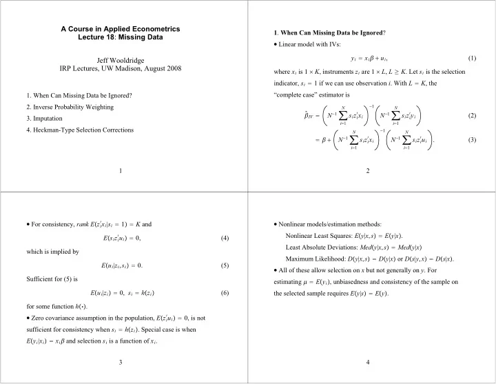
A Course in Applied Econometrics 1 . When Can Missing Data be Ignored ? Lecture 18 : Missing Data � Linear model with IVs: y i � x i � � u i , (1) Jeff Wooldridge IRP Lectures, UW Madison, August 2008 where x i is 1 � K , instruments z i are 1 � L , L � K . Let s i is the selection indicator, s i � 1 if we can use observation i . With L � K , the “complete case” estimator is 1. When Can Missing Data be Ignored? � 1 2. Inverse Probability Weighting N N N � 1 � N � 1 � � IV � � � x i � y i s i z i s i z i (2) 3. Imputation i � 1 i � 1 4. Heckman-Type Selection Corrections � 1 N N N � 1 � N � 1 � � x i � u i � � � s i z i s i z i . (3) i � 1 i � 1 1 2 � For consistency, rank E � z i � Nonlinear models/estimation methods: � x i | s i � 1 � � K and Nonlinear Least Squares: E � y | x , s � � E � y | x � . � u i � � 0, E � s i z i (4) Least Absolute Deviations: Med � y | x , s � � Med � y | x � which is implied by Maximum Likelihood: D � y | x , s � � D � y | x � or D � s | y , x � � D � s | x � . E � u i | z i , s i � � 0. (5) � All of these allow selection on x but not generally on y . For Sufficient for (5) is estimating � � E � y i � , unbiasedness and consistency of the sample on E � u i | z i � � 0, s i � h � z i � the selected sample requires E � y | s � � E � y � . (6) for some function h ��� . � Zero covariance assumption in the population, E � z i � u i � � 0, is not sufficient for consistency when s i � h � z i � . Special case is when E � y i | x i � � x i � and selection s i is a function of x i . 3 4

� Panel data: if we model D � y t | x t � , and s t is the selection indicator, the � If x it includes y i , t � 1 , (7) allows selection on y i , t � 1 , but not on “shocks” from t � 1 to t . sufficient condition to ignore selection is � Similar findings for NLS, quasi-MLE, quantile regression. D � s t | x t , y t � � D � s t | x t � , t � 1,..., T . (7) � Methods to remove time-constant, unobserved heterogeneity: for a Let the true conditional density be f t � y it | x it , � � . Then the partial random draw i , log-likelihood function for a random draw i from the cross section can y it � � t � x it � � c i � u it , (10) be written as with IVs z it for x it . Random effects IV methods (unbalanced panel): T T s it log f t � y it | x it , g � � � � s it l it � g � . (8) E � u it | z i 1 ,..., z iT , s i 1 ,..., s iT , c i � � 0, t � 1,..., T (11) t � 1 t � 1 Can show under (7) that E � c i | z i 1 ,..., z iT , s i 1 ,..., s iT � � E � c i � � 0. (12) E � s it l it � g � | x it � � E � s it | x it � E � l it � g � | x it � . (9) Selection in any time period cannot depend on u it or c i . 5 6 � FE on unbalanced panel: can get by with just (11). Let � Consistency of FE (and FEIV) on the unbalanced panel under breaks � 1 � r � 1 T ÿ it � y it � T i � it and z � it , where s ir y ir and similarly for and x down if the slope coefficients are random and one ignores this in estimation. The error term contains the term x i d i where d i � b i � � . T T i � � r � 1 s ir is the number of time periods for observation i . The FEIV Simple test based on the alternative estimator is E � b i | z i 1 ,..., z iT , s i 1 ,..., s iT � � E � b i | T i � . (13) � 1 N T N T N � 1 � N � 1 � � � � FEIV � � x � y it � s it z � it � it s it z � it . Then, add interaction terms of dummies for each possible sample size i � 1 t � 1 i � 1 t � 1 (with T i � T as the base group): T E � s it z � u it � � 0. Weakest condition for consistency is � t � 1 � it 1 � T i � 2 � x it , 1 � T i � 3 � x it , ..., 1 � T i � T � 1 � x it . (14) � One important violation of (11) is when units drop out of the sample Estimate equation by FE or FEIV. in period t � 1 because of shocks � u it � realized in time t . This generally induces correlation between s i , t � 1 and u it . Simple variable addition test. 7 8

� Can use FD in basic model, too, which is very useful for attrition 2 . Inverse Probability Weighting problems (later). Generally, if Weighting with Cross - Sectional Data � When selection is not on conditioning variables, can try to use � y it � � t � � x it � � u it , t � 2,..., T (15) probability weights to reweight the selected sample to make it and, if z it is the set of IVs at time t , we can use representative of the population. Suppose y is a random variable whose E � � u it | z it , s it � � 0 (16) population mean � � E � y � we would like to estimate, but some as being sufficient to ignore the missingess. Again, can add s i , t � 1 to test observations are missing on y . Let �� y i , s i , z i � : i � 1,..., N � indicate for attrition. independent, identically distributed draws from the population, where � Nonlinear models with unosberved effects are more difficult to z i is always observed (for now). handle. Certain conditional MLEs (logit, Poisson) can accomodate selection that is arbitrarily correlated with the unobserved effect. 9 10 � “Selection on observables” assumption � Sometimes p � z i � is known, but mostly it needs to be estimated. Let � � z i � denote the estimated selection probability: p P � s � 1| y , z � � P � s � 1| z � � p � z � (17) N � IPW � N � 1 � where p � z � � 0 for all possible values of z . Consider s i � y i . (19) � � z i � p i � 1 N � IPW � N � 1 � s i � y i , (18) p � z i � Can also write as i � 1 N � 1 � � where s i selects out the observed data points. Using (17) and iterated � � IPW � N 1 � s i y i (20) � � z i � p expectations, can show � � IPW is consistent (and unbiased) for y i . (Same i � 1 N s i is the number of selected observations and where N 1 � � i � 1 kind of estimate used for treatment effects.) � � � N 1 / N is a consistent estimate of P � s i � 1 � . 11 12

� A different estimate is obtained by solving the least squares problem � The HM problem is related to another issue. Suppose N E � y | x � � � � x � . (21) s i m � � y i � m � 2 . min � � z i � p Let z be a variables that are always observed and let p � z � be the i � 1 � Horowitz and Manski (1998) study estimating population means selection probability, as before. Suppose at least part of x is not always observed, so that x is not a subset of z . Consider the IPW estimator of � , using IPW. HM focus on bounds in estimating E � g � y � | x � A � for � solves conditioning variables x . Problem with certain IPW estimators based on weights that estimate P � s � 1 � / P � s � 1| z � : the resulting estimate of the N s i a , b � � y i � a � x i b � 2 . min (22) � � z i � p mean can lie outside the natural bounds. One should use i � 1 P � s � 1| x � A � / P � s � 1| x � A , z � if possible. Unfortunately, cannot generally estimate the proper weights if x is sometimes missing. 13 14 � The problem is that if � If selection is exogenous and x is always observed, is there a reason to use IPW? Not if we believe (21) along with the homoskedasticity P � s � 1| x , y � � P � s � 1| x � , (23) assumption Var � y | x � � � 2 . Then, OLS is efficient and IPW is less the IPW is generally inconsistent because the condition efficient. IPW can be more efficient with heteroskedasticity (but WLS P � s � 1| x , y , z � � P � s � 1| z � (24) with the correct heteroskedasticity function would be best). � Still, one can argue for weighting under (23) as a way to consistently is unlikely. On the other hand, if (23) holds, we can consistently estimate the parameters using OLS on the selected sample. estimate the linear projection. Write � If x always observed, case for weighting is much stronger because L � y |1, x � � � � � x � � (25) then x � z . If selection is on x , this should be picked up in large where L �� | �� denotes the linear projection. Under under samples in the estimation of P � s � 1| z � . P � s � 1| x , y � � P � s � 1| x � , the IPW estimator is consistent for � � . The unweighted estimator has a probabilty limit that depends on p � x � . 15 16