MUonE: how can lattice contribute? Marina Krsti Marinkovi Trinity - PowerPoint PPT Presentation
MUonE: how can lattice contribute? Marina Krsti Marinkovi Trinity College Dublin in collab. w. N. Cardoso (IST, Lisbon) and Second Plenary Workshop of the Muon g-2 Theory Initiative
MUonE: how can lattice contribute? Marina Krsti ć Marinkovi ć Trinity College Dublin in collab. w. N. Cardoso (IST, Lisbon) and Second Plenary Workshop of the Muon g-2 Theory Initiative JGU Mainz, 18-22 June 2018
MUonE: theoretical framework α ( t ) • Utilise the running of the fine-structure constant : Z 1 = α a had,LO dx (1 − x ) ∆ α had [ Q 2 ( x )] µ [Lautrup, de Rafael ‘69] π 0 ➡ In space-like (Euclidean) momenta region: Q 2 = x 2 m 2 µ 1 − x ➡ Measuring the Q 2 - dependent fine-structure constant: α ( O ) [ Phys.Lett. B746 (2015) 325-329 by Carloni, Passera,Trentadue, Venanzoni ] @ KLOE2 α ( Q 2 ) = 1 − ∆ α ( Q 2 ) [ Eur.Phys.J. C77 (2017) no.3, 139 by Abbiendi et al. ] Physics beyond colliders@CERN
MUonE: theoretical framework α ( t ) • Utilise the running of the fine-structure constant : Z 1 = α a had,LO dx (1 − x ) ∆ α had [ Q 2 ( x )] µ [Lautrup, de Rafael ‘69] π 0 ➡ In space-like (Euclidean) momenta region: Q 2 = x 2 m 2 µ 1 − x ➡ Measuring the Q 2 - dependent fine-structure constant: α ( O ) [ Phys.Lett. B746 (2015) 325-329 by Carloni, Passera,Trentadue, Venanzoni ] @ KLOE2 α ( Q 2 ) = 1 − ∆ α ( Q 2 ) [ Eur.Phys.J. C77 (2017) no.3, 139 by Abbiendi et al. ] Physics beyond colliders@CERN ➡ The running contributions can be split of the hadronic and leptonic part: ∆ α ( Q 2 ) = ∆ α had ( Q 2 ) + ∆ α lep ( Q 2 )
MUonE: theoretical framework α ( Q 2 ) ➡ MUonE will measure total : ∆ α ( Q 2 ) = ∆ α had ( Q 2 ) + ∆ α lep ( Q 2 ) Q 2 ∈ [0 . 001 , 0 . 14]GeV 2 ➡ Subtracting the purely leptonic part: Z 1 = α a had,LO dx (1 − x ) ∆ α had [ Q 2 ( x )] ∆ α ( Q 2 ) − ∆ α lep ( Q 2 ) ≡ ∆ α had ( Q 2 ) µ π 0 [Lautrup, de Rafael ‘69]
MUonE: theoretical framework α ( Q 2 ) ➡ MUonE will measure total : ∆ α ( Q 2 ) = ∆ α had ( Q 2 ) + ∆ α lep ( Q 2 ) Q 2 ∈ [0 . 001 , 0 . 14]GeV 2 ➡ Subtracting the purely leptonic part: Z 1 = α a had,LO dx (1 − x ) ∆ α had [ Q 2 ( x )] ∆ α ( Q 2 ) − ∆ α lep ( Q 2 ) ≡ ∆ α had ( Q 2 ) µ π 0 [Lautrup, de Rafael ‘69] experimental effort theoretical effort [NNLO amp.: Mastrolia et al. JHEP 11 (2017) 198 ] [NNLO had.: Brogio, Signer, Ulrich ] [NNLO+ Resumation Fael, Passera ] [MC@NNLO Pavia gr.,Czyz ] […]
MUonE: theoretical framework α ( Q 2 ) ➡ MUonE will measure total : ∆ α ( Q 2 ) = ∆ α had ( Q 2 ) + ∆ α lep ( Q 2 ) Q 2 ∈ [0 . 001 , 0 . 14]GeV 2 ➡ Subtracting the purely leptonic part: Z 1 = α a had,LO dx (1 − x ) ∆ α had [ Q 2 ( x )] ∆ α ( Q 2 ) − ∆ α lep ( Q 2 ) ≡ ∆ α had ( Q 2 ) µ π 0 [Lautrup, de Rafael ‘69] experimental known up to three loops [Steinhauser ‘98] effort for some Q 2 four loops [Baikov et al. ’13, Sturm ‘13] theoretical effort [NNLO amp.: Mastrolia et al. JHEP 11 (2017) 198 ] [NNLO had.: Brogio, Signer, Ulrich ] [NNLO+ Resumation Fael, Passera ] [MC@NNLO Pavia gr.,Czyz ] […]
MUonE: from the experimental region a HV P µ • MUonE: estimated precision for the HVP from the μ e exp. is 0.3% in [0,0.14]GeV 2 after two years of data taking [see slides by C. Carloni Calame, Thurs. 15.35] • Due to the experimental constraints: region [0.14, ∞ ] GeV 2 cannot be covered by the MUonE exp. | t | ( 10 − 3 GeV 2 ) Q 2 ≡ 0 0 . 55 2 . 98 10 . 5 35 . 7 ∞ 7 6 × 10 5 5 ⌘ µ ⇣ x 2 m 2 x − 1 4 (1 − x ) · ∆ α had 3 x max = 0 . 93 2 ➡ Q 2 = x 2 m 2 µ ➡ 1 1 − x Q 2 exp , max = 0 . 14GeV 2 ➡ 0 0 0 . 2 0 . 4 0 . 6 0 . 8 1 x max ∼ Q 2 x exp , max
MUonE: beyond the experimental region a HV P µ • MUonE: estimated precision for the HVP from the μ e exp. is 0.3% in [0,0.14]GeV 2 after two years of data taking [see slides by C. Carloni Calame, Thurs. 15.35] • Due to the experimental constraints: region [0.14, ∞ ] GeV 2 cannot be covered by the MUonE exp. | t | ( 10 − 3 GeV 2 ) Q 2 ≡ 0 0 . 55 2 . 98 10 . 5 35 . 7 ∞ 1. using time-like data from R-ratios / lattice QCD 7 Q 2 in [0.14GeV 2 , Q 2high ] 6 × 10 5 pQCD Q 2 in [Q 2high , ∞ ] 2. 5 ⌘ µ ⇣ x 2 m 2 x − 1 4 (1 − x ) · ∆ α had 3 x max = 0 . 93 2 ➡ Q 2 = x 2 m 2 µ ➡ 1 1 − x Q 2 exp , max = 0 . 14GeV 2 ➡ 0 0 0 . 2 0 . 4 0 . 6 0 . 8 1 x max ∼ Q 2 x exp , max
MUonE: beyond the experimental region a HV P µ • MUonE: estimated precision for the HVP from the μ e exp. is 0.3% in [0,0.14]GeV 2 after two years of data taking [see slides by C. Carloni Calame, Thurs. 15.35] • Due to the experimental constraints: region [0.14, ∞ ] GeV 2 cannot be covered by the MUonE exp. Z 0 . 93 ... ⌘ 2 Z Q 2 ⌘ 2 Z ∞ ⇣ α = α max ⇣ α dQ 2 f ( Q 2 ) × ˆ dQ 2 f ( Q 2 ) × ˆ a had,LO dx (1 − x ) ∆ α had [ Q 2 ( x )] + Π ( Q 2 )+ Π pert. ( Q 2 ) µ π π π Q 2 0 0 . 14 max | {z } I 0
MUonE: beyond the experimental region a HV P µ • MUonE: estimated precision for the HVP from the μ e exp. is 0.3% in [0,0.14]GeV 2 after two years of data taking [see slides by C. Carloni Calame, Thurs. 15.35] • Due to the experimental constraints: region [0.14, ∞ ] GeV 2 cannot be covered by the MUonE exp. Z 0 . 93 ... ⌘ 2 Z Q 2 ⌘ 2 Z ∞ ⇣ α = α max ⇣ α dQ 2 f ( Q 2 ) × ˆ dQ 2 f ( Q 2 ) × ˆ a had,LO dx (1 − x ) ∆ α had [ Q 2 ( x )] + Π ( Q 2 )+ Π pert. ( Q 2 ) µ π π π Q 2 0 0 . 14 max | {z } I 1 • lattice QCD • R-ratios
MUonE: beyond the experimental region a HV P µ • MUonE: estimated precision for the HVP from the μ e exp. is 0.3% in [0,0.14]GeV 2 after two years of data taking [see slides by C. Carloni Calame, Thurs. 15.35] • Due to the experimental constraints: region [0.14, ∞ ] GeV 2 cannot be covered by the MUonE exp. Z 0 . 93 ... ⌘ 2 Z Q 2 ⌘ 2 Z ∞ ⇣ α ⇣ α = α max dQ 2 f ( Q 2 ) × ˆ dQ 2 f ( Q 2 ) × ˆ a had,LO dx (1 − x ) ∆ α had [ Q 2 ( x )] + Π ( Q 2 )+ Π pert. ( Q 2 ) µ π π π Q 2 0 0 . 14 max | {z } I 2 [Chetyrkin et al. ‘96] [Harlander&Steinhauser ‘02] + matching term (I 3 )… [see e.g. BMW arXiv:1711.04980 ] [K. Miura, Thurs. 9.00]
MUonE: beyond the experimental region a HV P µ • MUonE: estimated precision for the HVP from the μ e exp. is 0.3% in [0,0.14]GeV 2 after two years of data taking [see slides by C. Carloni Calame, Thurs. 15.35] • Due to the experimental constraints: region [0.14, ∞ ] GeV 2 cannot be covered by the MUonE exp. Z 0 . 93 ... ⌘ 2 Z Q 2 ⌘ 2 Z ∞ ⇣ α = α max ⇣ α dQ 2 f ( Q 2 ) × ˆ dQ 2 f ( Q 2 ) × ˆ a had,LO dx (1 − x ) ∆ α had [ Q 2 ( x )] + Π ( Q 2 )+ Π pert. ( Q 2 ) µ π π π Q 2 0 0 . 14 max | {z } I 1 • lattice QCD • R-ratios
Phys. Rev. D 90, 074508 (2014), Hybrid method [Golterman,Maltman,Peris] • Low momentum region ➡ Experiment (NLO, NNLO, radiative corrections … )
Phys. Rev. D 90, 074508 (2014), Hybrid method [Golterman,Maltman,Peris] • Low momentum region ➡ Experiment (NLO, • Vary low and high Q 2 cut NNLO, radiative corrections … )
Phys. Rev. D 90, 074508 (2014), Hybrid method [Golterman,Maltman,Peris] • Low momentum region ➡ Experiment (NLO, • Vary low and high Q 2 cut NNLO, radiative corrections … ) ➡ continuum limit: a—> 0 ➡ infinite volume limit: V—> ∞ ➡ physical quark masses ➡ isospin breaking corrections (m u ≠ m d and α em ≠ 0)
Phys. Rev. D 90, 074508 (2014), Hybrid method [Golterman,Maltman,Peris] • Low momentum region ➡ Experiment (NLO, • Vary low and high Q 2 cut NNLO, radiative corrections … ) ➡ continuum limit: a—> 0 (0.049-0.076fm) infinite volume limit: V—> ∞ ➡ ➡ physical quark masses (extrap. m π ≈ 270-440MeV) ➡ isospin breaking corrections (m u ≠ m d and α em ≠ 0)
Hybrid method: from experimental + lattice QCD data 120 [0.14,4.0]GeV 2 x 10 10 cont. limit cont. limit 2 + α 3 m π 2 ln (m π 2 ) α 1 + α 2 m π 2 + α 3 m π 2 ln (m π 2 ) α 1 + α 2 m π 100 P r e l 80 i m i n a r y 60 had,LO 40 I1 = a µ 20 0 2 0 0.05 0.1 0.15 0.2 m π ,phys 2 [GeV 2 ] m π
Hybrid method: from experimental + lattice QCD data 120 [0.14,4.0]GeV 2 x 10 10 cont. limit cont. limit 2 + α 3 m π 2 ln (m π 2 ) α 1 + α 2 m π 2 + α 3 m π 2 ln (m π 2 ) α 1 + α 2 m π 100 P r e l 80 i m i n a r y 60 had,LO 40 I1 = a µ 20 0 2 0 0.05 0.1 0.15 0.2 m π ,phys 2 [GeV 2 ] m π ➡ Nf=2, A5,E5,F6,N6,O7 (CLS), m π ≈ 270-440MeV ➡ u,d,s,c connected, no isospin breaking corr. Π (0) = − ∂ Π 12 ( Q ) | Q 2 =0 ➡ [de Divitiis et al., Phys.Lett. B718 (2012)] ∂ Q 1 ∂ Q 2 Pade fits [0.14, 4.0] GeV 2 (to be compared with numerical integration/conformal pol. fits in the low-Q 2 ) ➡ ➡ Continuum + chiral extrapolation [arXiv:1705.01775]: α 1 + α 2 m 2 π + α 3 m 2 π ln ( m 2 π ) + α 4 a ➡ Preliminary result with 9.7% uncertainty on I1, more statistics and one more m π underway ➡ Possible improvements: diff. chiral extrap. + improved vector current [H. Meyer, Wed. 16.30]
Recommend
More recommend
Explore More Topics
Stay informed with curated content and fresh updates.
