Multivariate option pricing models: some extensions of the VG model - PowerPoint PPT Presentation
Multivariate option pricing models: some extensions of the VG model Florence Guillaume Actuarial and Financial Statistics workshop, Eindhoven August 29th-30th, 2011 1 / 41 Time change in finance time-changed Brownian motion W ( T ( t )) in
Multivariate option pricing models: some extensions of the α VG model Florence Guillaume Actuarial and Financial Statistics workshop, Eindhoven August 29th-30th, 2011 1 / 41
Time change in finance time-changed Brownian motion W ( T ( t )) in finance: first proposed by Clark (1973) ⇒ Business clock T ( t ) (positive stochastic process) quantifies the information arrival rate Motivation: information flow directly affects evolution of the price: when low amount of available information, slow trading and price process evolves slowly time change T : characteristics no loss of information over time ⇒ non decreasing process amount of new information independent on the amount of information previously released ⇒ independent increments amount of released information during [ t , t + dt ] only depends on the length of that interval dt ⇒ stationary increments ⇒ T ≡ subordinator (non-decreasing L´ evy process) 2 / 41
L´ evy processes Definition X = { X t , t ≥ 0 } defined on (Ω , F , P ) is a L´ evy process if X starts at 0: X 0 = 0 a.s.; X has independent increments; X has stationary increments. ⇒ X t + s − X s ∼ infinitely divisible distribution and has ( φ ( u )) t as CF, where φ ( u ) is the CF of X 1 . Definition L´ evy-Khintchine representation of an infinitely divisible distribution CF: � + ∞ log( φ X ( u )) = i γ u − σ 2 2 u 2 + � � exp( iux ) − 1 − iux 1 | x | < 1 ν ( dx ) −∞ where γ ∈ R , σ 2 ≥ 0 and ν is a measure on R \ { 0 } satisfying � + ∞ 1 , x 2 � � −∞ inf ν ( dx ) < ∞ 3 / 41
Example: the VG process as time-changed Brownian motion (BM) The Gamma process CF of Gamma( a , b ) with a > 0, b > 0: � − a � 1 − i u φ Gamma ( u ; a , b ) = b Scaling property : if X ∼ Gamma( a , b ) then cX ∼ Gamma( a , b / c ) , c > 0 (1) X t ∼ Gamma( at , b ) (2) If X i ∼ Gamma( a i , b ) are N independent r.v. then � N N � � � X i ∼ Gamma a i , b (3) i =1 i =1 4 / 41
Example: the VG process as time-changed Brownian motion (Cont) The VG process VG( σ, ν, θ ) process ≡ Gamma time-changed BM with drift X VG ( σ, ν, θ ) = θ G t + σ W G t t where G = { G t , t ≥ 0 } ∼ Gamma ( t /ν, 1 /ν ) process and W = { W t , t ≥ 0 } is a standard Brownian motion CF of VG ( σ, ν, θ ) with σ > 0, ν > 0, θ ∈ R : 1 − i u θν + u 2 σ 2 ν � − 1 � ν φ VG ( u ; σ, ν, θ ) = 2 VG ( σ, ν, θ ) VG ( σ, ν, 0) mean θ 0 σ 2 + νθ 2 σ 2 variance � 3 σ 2 +2 νθ 2 � θν skewness 0 σ 2 + νθ 2 � 3 � 2 � � νσ 4 kurtosis 3 1 + 2 ν − 3(1 + ν ) ( σ 2 + νθ 2 ) 2 5 / 41
Multivariate L´ evy models as time changed BM 1 multivariate BM subordinated by an univariate time change (Madan and Senata, 1990). Unique business clock ⇒ independence can not be captured 2 α VG model (Semeraro, 2008): extend multivariate time changed BM by considering a subordinator = sum of idiosyncratic and common Gamma subordinators: G ( i ) = X ( i ) + α i Z t t t Original model: constraints on the Gamma subordinator parameters such that G ( i ) ∼ Gamma . CFs: independent of 1 common subordinator settings ⇒ calibration requires multivariate derivatives 3 multivariate L´ evy two factors models (Luciano and Semeraro, 2010): extend the α VG model to other subordinator distributions 6 / 41
Some extensions of the α VG model 1 relax the constraints imposed on the subordinator parameters in the original model 2 consider Sato processes instead of L´ evy processes 7 / 41
The α VG model S (1) � ( r − q 1 ) t + Y (1) � exp 0 t � � �� Y (1) exp E S (1) t t � � S (2) ( r − q 2 ) t + Y (2) exp S (2) t 0 S t = t = � � Y (2) �� E exp t . . . . . . S ( N ) � � S ( N ) ( r − q N ) t + Y ( N ) t exp 0 t � � �� Y ( N ) E exp t θ 1 G (1) + σ 1 W (1) Y (1) G (1) X (1) t G (1) + α 1 Z t t t t t θ 2 G (2) + σ 2 W (2) Y (2) G (2) X (2) + α 2 Z t t G (2) t t t Y t = = G t = = t . . . . . . . . . . . . Y ( N ) G ( N ) X ( N ) θ N G ( N ) + σ N W ( N ) + α N Z t t t t t G ( N ) t where W ( i ) ’s are independent standard BM, α i > 0, Z 1 ∼ Gamma ( c 1 , c 2 ) , c 1 , c 2 > 0 and X ( i ) ∼ Gamma ( a i , b i ), a i , b i > 0 1 are independent r.v. and are independent of the W ( i ) ’s. 8 / 41
The α VG model: CF’s CF of Y t : N � u i θ i + i1 � exp(i u ′ Y t ) � 2 σ 2 i u 2 � � φ Y ( u , t ) = E = φ X ( i ) i , t 1 i =1 � N � � u i θ i + i1 � � 2 σ 2 i u 2 φ Z 1 α i , t i i =1 marginal CF’s � − a i t � � �� − c 1 t 1 − i u θ i + i 1 2 σ 2 i u 2 � 1 − i α i u θ i + i1 2 σ 2 i u 2 φ Y ( i ) ( u , t ) = b i c 2 c 2 = 1 (by space scaling property (1)) On average, business time grows as the real time: � � G ( i ) = t ⇒ a i b i = 1 − α i c 1 (4) ⇒ E t c 2 � � c 1 b i 1 − α i > 0 ( 5 ) c 2 9 / 41
The α VG model: correlation � � Y ( i ) t , Y ( j ) Cov t ρ ij = � � � � � Y ( i ) Y ( j ) Var Var t t where � � Y ( i ) t , Y ( j ) = θ i θ j α i α j c 1 Cov 2 t t c 2 � � � � � � �� Y ( i ) θ 2 a i i + α 2 c 1 + σ 2 a i b i + α i c 1 Var = t t b 2 c 2 i i i c 2 2 ⇒ time independent correlations 10 / 41
The original α VG model Original α VG model : impose b i = c 2 ∀ i such that α i (4) (3) G ( i ) ∼ Gamma( a i + c 1 , c 2 ≡ Gamma( c 2 α i , c 2 α i ) α i ) ⇒ 1 �� − c 2 α i t � 1 − i α i � u θ i + i1 2 σ 2 i u 2 φ Y ( i ) ( u , t ) = c 2 � σ i , α i � ⇒ Y ( i ) ∼ VG , θ i 1 c 2 ⇒ CFs independent of the common subordinator setting θ i θ j α i α j ρ ij = � c 1 ∝ c 1 . �� θ 2 � � θ 2 b i + σ 2 b j + σ 2 j i i j 11 / 41
The generalized α VG model Generalized α VG model : relax the constraints on the b i ’s ⇒ � − a i t � � i u 2 �� − c 1 t u θ i + i 1 2 σ 2 i u 2 1 − i α i � u θ i + i 1 2 σ 2 φ Y ( i ) ( u , t ) = 1 − i b i c 2 = ( φ Y ( i ) ( u , 1)) t ⇒ CFs depend on the whole parameter set Y ( i ) ∼ L´ evy process (but not necessarily VG) t 12 / 41
Towards the Sato two factors models Extend the two factors L´ evy model to the class of Sato processes: Sato processes typically lead to a significantly better fit of option prices in both the strike and time to maturity dimensions in the univariate case (Carr, Geman, Madan and Yor, 2007) 13 / 41
Sato processes Definition X is self-decomposable if X d = cX + X c , ∀ 0 < c < 1 , where X c is independent of X. Self-decomposable distributions are infinitely divisible distributions with a L´ evy-Khintchine representation � + ∞ log Φ X ( u ) = i γ u − σ 2 � h ( x ) 2 u 2 + � exp(i ux ) − 1 − i ux 1 | x | < 1 | x | dx −∞ where h ( x ) ≥ 0 is decreasing for x > 0 and increasing for x < 0. The probability law of the Sato process at time t is obtained by scaling the self-decomposable law of X at unit time: d = t γ X , X t where γ = self-similar exponent. Sato processes have independent but time inhomogeneous increments. 14 / 41
The Sato VG process From the L´ evy density of the VG process, � C exp( Gx ) x < 0 , dx | x | ν VG ( dx ) = C exp( − Mx ) dx x > 0 , | x | the VG probability law at unit time is self-decomposable for all acceptable VG parameter sets { σ, ν, θ } . CF of VG Sato process at time t : X VG Sato ( σ, ν, θ, γ ) = t γ X VG ( σ, ν, θ ) t 1 φ VG Sato ( u , t ; σ, ν, θ, γ ) = φ VG ( u , 1; t γ σ, ν, t γ θ ) � − 1 ν . � 1 − i u νθ t γ + σ 2 ν t 2 γ u 2 = 2 15 / 41
The Sato α VG model θ 1 t γ 1 G (1) + σ 1 t γ 1 W (1) Y (1) t G (1) θ 2 t γ 2 G (2) + σ 2 t γ 2 W (2) Y (2) t Y t = = G (2) . . . . . . Y ( N ) θ N t γ N G ( N ) + σ N t γ N W ( N ) t G ( N ) X (1) + α 1 Z G (1) X (2) + α 2 Z G (2) G = = . . . . . . X ( N ) + α N Z G ( N ) where W ( i ) ’s are independent standard BM, α i > 0, Z ∼ Gamma ( c 1 , c 2 ) , c 1 , c 2 > 0 and X ( i ) ∼ Gamma ( a i , b i ), a i , b i > 0 are independent random variables and are independent of the W ( i ) ’s. 16 / 41
The Sato α VG model (Cont) CF of Y t : N � � u i θ i t γ i + i 1 φ Y ( u , t ) = E [exp( iu ′ Y t )] � 2 σ 2 i t 2 γ i u 2 = φ X ( i ) i i =1 � N �� � u i θ i t γ i + i 1 � 2 σ 2 i t 2 γ i u 2 φ Z 1 α i . i i =1 marginal CF’s � − a i � � 1 − i u θ i t γ i + i 1 2 σ 2 i t 2 γ i u 2 �� − c 1 1 − i α i � u θ i t γ i + i 1 2 σ 2 i t 2 γ i u 2 φ Y ( i ) ( u , t ) = b i c 2 c 2 = 1 � � G ( i ) � = 1 ⇒ a i b i = 1 − α i c 1 1 − α i c 1 � c 2 ⇒ b i > 0 E c 2 17 / 41
Recommend
More recommend
Explore More Topics
Stay informed with curated content and fresh updates.
