Multigrid for Poissons Equation Prof. Richard Vuduc Georgia - PowerPoint PPT Presentation
Multigrid for Poissons Equation Prof. Richard Vuduc Georgia Institute of Technology CSE/CS 8803 PNA, Spring 2008 [L.12] Thursday, February 14, 2008 1 Sources for todays material CS 267 (Yelick & Demmel, UCB) Applied Numerical Linear
Multigrid for Poisson’s Equation Prof. Richard Vuduc Georgia Institute of Technology CSE/CS 8803 PNA, Spring 2008 [L.12] Thursday, February 14, 2008 1
Sources for today’s material CS 267 (Yelick & Demmel, UCB) Applied Numerical Linear Algebra , by Demmel Heath (UIUC) 2
Review: Parallel FFT 3
Exploiting structure to obtain fast algorithms for 2-D Poisson Dense LU : Assume no structure ⇒ O(n 6 ) Sparse LU : Sparsity ⇒ O(n 3 ), need extra memory CG : Symmetric positive definite ⇒ O(n 3 ), a little extra memory RB SOR : Fixed sparsity pattern ⇒ O(n 3 ), no extra memory FFT : Eigendecomposition ⇒ O(n 2 log n) 4
Fast Fourier transform algorithm FFT( x, ω , m ) if m == 1 then return x 0 else x even ← FFT( x even , ω 2 , m 2 ) x odd ← FFT( x odd , ω 2 , m 2 ) m w 0 , w 1 , . . . , ω 2 − 1 � � = precomputed w ← ⇐ � � x even + ( w. ∗ x odd) , x even − ( w. ∗ x odd) return 5
0000 0001 0010 0011 0100 0101 0110 0111 1000 1001 1010 1011 1100 1101 1110 1111 log p: No comm log (m/p): No comm FFT with transpose (p=4) 6
Algorithms for 2-D (3-D) Poisson, N=n 2 (=n 3 ) Algorithm Serial PRAM Memory # procs Dense LU N 3 N N 2 N 2 Band LU N 2 (N 7/3 ) N N 3/2 (N 5/3 ) N (N 4/3 ) Jacobi N 2 (N 5/3 ) N (N 2/3 ) N N Explicit inverse N 2 log N N 2 N 2 Sparse LU N 3/2 (N 2 ) N 1/2 N log N (N 4/3 ) N Conj. grad. N 3/2 (N 4/3 ) N 1/2(1/3) log N N N RB SOR N 3/2 (N 4/3 ) N 1/2 (N 1/3 ) N N FFT N log N log N N N Multigrid N log 2 N N N N log N N Lower bound PRAM = idealized parallel model with zero communication cost. Source: Demmel (1997) 7
Recall: Discretizing 2-D Poisson Graph and stencil 2 4 5 6 8 4 − 1 − 1 1 4 7 − 1 4 − 1 − 1 − 1 4 − 1 − 1 4 − 1 − 1 2 5 8 − 1 − 1 4 − 1 − 1 − 1 − 1 4 − 1 3 6 9 − 1 4 − 1 − 1 − 1 4 − 1 − 1 − 1 4 4 u ij − u i +1 ,j − u i − 1 ,j − u i,j +1 − u i,j − 1 = h 2 f i,j 8
Recall: Jacobi’s method Rearrange terms in (2-D) Poisson: u i,j = 1 u i − 1 ,j + u i +1 ,j + u i,j − 1 + u i,j +1 + h 2 f i,j � � 4 For each (i, j), iteratively update (weighted averaging): = 1 � � u ( t +1) u ( t ) i − 1 ,j + u ( t ) i +1 ,j + u ( t ) i,j − 1 + u ( t ) i,j +1 + h 2 f i,j i,j 4 Motivation: Match solution to discrete Poisson exactly at nodes. 9
Problem: Slow convergence RHS True solution 5 steps of Jacobi Best possible 5-step 10
Recall: Convergence of Jacobi’s method Converges in O(N=n 2 ) steps, so serial complexity is O(N 2 ) . Define error at each step as: �� ǫ t � ( u t i,j − u i,j ) 2 i,j For Jacobi, can show: � t 1 − π 2 � � � 4 · t π n →∞ cos ǫ t ≤ ≈ ǫ 0 ǫ 0 n 2 n + 1 11
Consider Jacobi in 1-D h 2 f i − u i − 1 + 2 u i − u i +1 = + h 2 � � 1 u ( t +1) u ( t ) i − 1 + u ( t ) 2 f i = i +1 i 2 ⇓ � � · u ( t ) + h 2 I − 1 u ( t +1) 2 T n 2 f = � �� � ≡ R R · u ( t ) + c ≡ 12
Closer look at 1-D Jacobi’s convergence Consider total error at each step ǫ ( t ) u ( t ) − u ≡ R · ǫ ( t − 1) = R t · e 0 = 13
Closer look at 1-D Jacobi’s convergence Consider slightly broader class of weighted Jacobi methods h 2 f ≡ c T n u = I − w R w ≡ 2 T n R w u ( t ) + w u ( t +1) 2 c = ⇓ ǫ ( t ) w ǫ (0) R t = 14
1-D Poisson: Eigendecomposition of T n Lemma : Eigenvalues and eigenvectors of T n are Z Λ Z T = T n T n z j λ j z j ⇒ = = ZZ T I = � � π j = 2 1 − cos λ j n + 1 � 2 n + 1 sin π jk z j ( k ) = n + 1 15
Error “frequencies” ( I − w ǫ ( t ) = R t 2 Z Λ Z T ) t · ǫ (0) w · ǫ (0) = I − w � t � Z T · ǫ (0) = 2 Λ Z ⇓ I − w � t � Z T · ǫ ( t ) Z T · ǫ (0) = 2 Λ I − w � t � Z T · ǫ ( t ) � � � Z T · ǫ (0) � = 2 Λ j j jj 16
Spectrum of R_w 1.00 0.75 w =1/2 0.50 0.25 0 w =2/3 -0.25 -0.50 w =1 -0.75 -1.00 j=n/2 For 1-D discrete Poisson, with n = 99 17
Initial error “Rough” Lots of high frequency components Norm = 1.65 Error after 1 weighted Jacobi step “Smoother” Less high frequency component Norm = 1.06 Error after 2 weighted Jacobi steps “Smooth” Little high frequency component Norm = .92, won’t decrease much more 18
Faster information propagation? “Multigrid” idea Approximate problem on fine grid by a coarser grid Solve the coarse grid problem approximately Interpolate coarse grid solution onto fine grid, as an initial guess Recursively solve coarse grid problems To work, coarse grid solution must be a good approximation to fine grid 19
Same idea applies elsewhere Multilevel graph partitioning (METIS) Coarsen graph via maximal independent set problem Partition coarse graph, refine using Kernighan-Lin Barnes-Hut and fast multipole method for, say, gravity problems Approximate particles in a region by total mass, center of gravity Divide regions recursively 20
Divide-and-conquer in multigrid Spatial domain Get an initial solution for an n × n grid by solving approximately on n/2 × n/2 grid Recurse Frequency domain Think of error as sum of eigenvectors, e.g. , sine-curves of different frequencies Solving on a particular grid “smooths” (dampens) high-frequency error 21
“Multigrids” in 1-D Problem on 2 i + 1 grid P ( i ) = T ( i ) x ( i ) b ( i ) = P (3) P (2) P (1) 22
“Multigrids” in 2-D 2 i + 1 2 i + 1 P ( i ) � � � � = Problem on grid × T ( i ) x ( i ) b ( i ) = P (3) P (2) P (1) 23
Multigrid operators P (3) Restrict(3) P (2) Restrict(2) P (1) P (3) Interpolate(2) P (2) Interpolate(1) P (1) 24
Multigrid operators P ( i ) : x ( i ) Current estimated solution ≡ b ( i ) Right-hand side ≡ b ( i − 1) ← R ( i ) � b ( i ) � ⇐ Restriction R ( i ) : x ( i ) ← L ( i − 1) � x ( i − 1) � L ( i ) ⇐ Interpolation : improved ← S ( i ) � b ( i ) , x ( i ) � x ( i ) S ( i ) : ⇑ Solution operator (smoother) 25
Multigrid “V-cycle”: Building block for the full multigrid algorithm � b ( i ) , x ( i ) � ⇐ Returns improved x (i) for T (i) x (i) = b (i) MGV if i == 1 then i Calls & returns return exact solution of P (1) 5 else x ( i ) ← S ( i ) � b ( i ) , x ( i ) � 4 r ( i ) ← T ( i ) · x ( i ) − b ( i ) 3 d ( i ) ← L ( i − 1) � � R ( i ) � r ( i ) � �� MGV , 0 2 x ( i ) ← x ( i ) − d ( i ) x ( i ) ← S ( i ) � b ( i ) , x ( i ) � 1 time return x ( i ) 26
Multigrid V-cycle � b ( i ) , x ( i ) � ⇐ Returns improved x (i) for T (i) x (i) = b (i) MGV if i == 1 then return exact solution of P (1) Base case: 1 unknown else x ( i ) ← S ( i ) � b ( i ) , x ( i ) � r ( i ) ← T ( i ) · x ( i ) − b ( i ) d ( i ) ← L ( i − 1) � � R ( i ) � r ( i ) � �� MGV , 0 x ( i ) ← x ( i ) − d ( i ) x ( i ) ← S ( i ) � b ( i ) , x ( i ) � return x ( i ) 27
Multigrid V-cycle � b ( i ) , x ( i ) � ⇐ Returns improved x (i) for T (i) x (i) = b (i) MGV if i == 1 then return exact solution of P (1) Base case: 1 unknown else x ( i ) ← S ( i ) � b ( i ) , x ( i ) � Smooth (damps high-freq error) r ( i ) ← T ( i ) · x ( i ) − b ( i ) d ( i ) ← L ( i − 1) � � R ( i ) � r ( i ) � �� MGV , 0 x ( i ) ← x ( i ) − d ( i ) x ( i ) ← S ( i ) � b ( i ) , x ( i ) � return x ( i ) 28
Multigrid V-cycle � b ( i ) , x ( i ) � ⇐ Returns improved x (i) for T (i) x (i) = b (i) MGV if i == 1 then return exact solution of P (1) Base case: 1 unknown else x ( i ) ← S ( i ) � b ( i ) , x ( i ) � Smooths (damps high-freq error) Computes residual r ( i ) ← T ( i ) · x ( i ) − b ( i ) d ( i ) ← L ( i − 1) � � R ( i ) � r ( i ) � �� Recursively solves MGV , 0 x ( i ) ← x ( i ) − d ( i ) Corrects fine-grid solution x ( i ) ← S ( i ) � b ( i ) , x ( i ) � return x ( i ) 29
Multigrid V-cycle � b ( i ) , x ( i ) � ⇐ Returns improved x (i) for T (i) x (i) = b (i) MGV if i == 1 then return exact solution of P (1) Base case: 1 unknown else x ( i ) ← S ( i ) � b ( i ) , x ( i ) � Smooths (damps high-freq error) Computes residual r ( i ) ← T ( i ) · x ( i ) − b ( i ) d ( i ) ← L ( i − 1) � � R ( i ) � r ( i ) � �� Recursively solves MGV , 0 x ( i ) ← x ( i ) − d ( i ) Corrects fine-grid solution x ( i ) ← S ( i ) � b ( i ) , x ( i ) � Smooth again return x ( i ) 30
Multigrid V-cycle � b ( i ) , x ( i ) � ⇐ Returns improved x (i) for T (i) x (i) = b (i) MGV if i == 1 then i Calls & returns return exact solution of P (1) 5 else x ( i ) ← S ( i ) � b ( i ) , x ( i ) � 4 r ( i ) ← T ( i ) · x ( i ) − b ( i ) 3 d ( i ) ← L ( i − 1) � � R ( i ) � r ( i ) � �� MGV , 0 2 x ( i ) ← x ( i ) − d ( i ) x ( i ) ← S ( i ) � b ( i ) , x ( i ) � 1 time return x ( i ) 31
Multigrid V-cycle: Correction step . . . r ( i ) ← T ( i ) · x ( i ) − b ( i ) d ( i ) ← L ( i − 1) � � R ( i ) � r ( i ) � �� MGV , 0 x ( i ) ← x ( i ) − d ( i ) . . . Justification: T ( i ) d ( i ) r ( i ) = T ( i ) x ( i ) − b ( i ) = T ( i ) � x ( i ) − d ( i ) � ⇒ b ( i ) = = 32
Recommend
More recommend
Explore More Topics
Stay informed with curated content and fresh updates.
