Moving Average Model Moving average model of order q (MA( q )): x t - - PowerPoint PPT Presentation

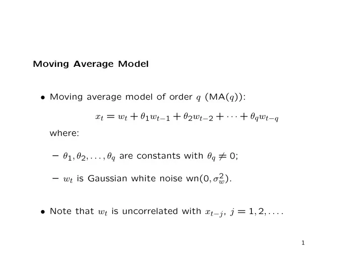
Moving Average Model

• Moving average model of order q (MA(q)):

xt = wt + θ1wt−1 + θ2wt−2 + · · · + θqwt−q where: – θ1, θ2, . . . , θq are constants with θq = 0; – wt is Gaussian white noise wn(0, σ2

w).

• Note that wt is uncorrelated with xt−j, j = 1, 2, . . . .

1

• In operator form:

xt = θ(B)wt, where the moving average operator θ(B) is θ(B) = 1 + θ1B + θ2B2 + · · · + θqBq.

• Compare with the autoregressive model φ(B)xt = wt.
• The moving average process is stationary for any values of

θ1, θ2, . . . , θq.

2

Moments

• Mean: E (xt) = 0.
• Autocovariances:

γ(h) = cov

• xt+h, xt
• = E

   

j

θjwt+h−j

   

k

θkwt−k

   

= σ2

w

• k

θkθk+h = 0 if h > q.

3

• The MA(q) model is characterized by

γ(q) = σ2

wθq = 0

γ(h) = 0 for h > q.

• The contrast between the ACF of

– a moving average model, which is zero except for a finite number of lags h – an autoregressive model, which goes to zero geometrically makes the sample ACF an important tool in deciding what model to fit.

4

Inversion

• Example: MA(1)

xt = wt + θwt−1 = (1 + θB)wt, so if |θ| < 1, wt = (1 + θB)−1xt = π(B)xt, where π(B) =

∞

• j=0

(−θ)jBj.

• So xt satisfies an infinite autoregression:

xt =

∞

• j=1

−(−θ)jxt−j + wt,

5

Autoregressive Moving Average Models

• Combine! ARMA(p, q):

xt =φ1xt−1 + φ2xt−2 + · · · + φpxt−p + wt + θ1wt−1 + θ2wt−2 + · · · + θqwt−q.

• In operator form:

φ(B)xt = θ(B)wt.

6

Issues in ARMA Models Parameter redundancy: if φ(z) and θ(z) have any common fac- tors, they can be canceled out, so the model is the same as

• ne with lower orders. We assume no redundancy.

Causality: If φ(z) = 0 for |z| ≤ 1, xt can be written in terms of present and past ws. We assume causality. Invertibility: If θ(z) = 0 for |z| ≤ 1, wt can be written in terms

• f present and past xs, and xt can be written as an infinite
• autoregression. We assume invertibility.

7

Using proc arima

• Example: fit an MA(1) model to the differences of the log

varve thicknesses.

• options linesize = 80;
• ds html file = ’../varve1.html’;

data varve; infile ’../data/varve.dat’; input varve; lv = log(varve); dlv = dif(lv); run;

8

proc arima data = varve; title ’Fit an MA(1) model to differences of log varve’; identify var = dlv; estimate q = 1; run;

• proc arima output

Using some proc arima options

• Example: fit an IMA(1) model to the log varve thicknesses.
• options linesize = 80;
• ds html file = ’varve2.html’;

data varve; infile ’varve.dat’; input varve; lv = log(varve); run;

9

proc arima data = varve; title ’Fit an IMA(1, 1) model to log varve, using ML’; title2 ’Use minic option to identify a good model’; identify var = lv(1) minic; estimate q = 1 method = ml; estimate q = 2 method = ml; estimate p = 1 q = 1 method = ml; run;

• proc arima output

Notes on the proc arima output

• For the MA(1) model, the “Autocorrelation Check of Resid-

uals” rejects the null hypothesis that the residuals are white noise. – If the series really had MA(1) structure, the residuals would be white noise. – So the MA(1) model is not a good fit for this series.

• For both the MA(2) and the ARMA(1, 1) models, the “Chi-

Square” statistics are not significant, so these models both seem satisfactory. ARMA(1, 1) has the better AIC and SBC.

10

Using R

• Fit a given model and test the residuals as white noise:

varve.ma1 = arima(diff(log(varve)),

• rder = c(p = 0, d = 0, q = 1));

varve.ma1; Box.test(residuals(varve.ma1), lag = 6, type = "Ljung", fitdf = 1);

• Note: the fitdf argument indicates that these are residuals

from a fit with a single parameter.

11

• As in proc arima, differencing can be carried out within arima():

varve.ima1 = arima(log(varve), order = c(0, 1, 1)); varve.ima1; Box.test(residuals(varve.ima1), 6, "Ljung", 1);

• But note that you cannot include the intercept, so the results

are not identical. – Rerun the original analysis with no intercept: arima(diff(log(varve)), order = c(0, 0, 1), include.mean = FALSE);

12

• Make a table of AICs:

AICtable = matrix(NA, 5, 5); dimnames(AICtable) = list(paste("p =", 0:4), paste("q =", 0:4)); for (p in 0:4) { for (q in 0:4) { varve.arma = arima(diff(log(varve)), order = c(p, 0, q)); AICtable[p+1, q+1] = AIC(varve.arma); } } AICtable;

• Note: proc arima’s MINIC option tabulates (an approximation

to) BIC, not AIC.

13

• Make a table of BICs:

BICtable = matrix(NA, 5, 5); dimnames(BICtable) = list(paste("p =", 0:4), paste("q =", 0:4)); for (p in 0:4) { for (q in 0:4) { varve.arma = arima(diff(log(varve)), order = c(p, 0, q)); BICtable[p+1, q+1] = AIC(varve.arma, k = log(length(varve) - 1)); } } BICtable;

• Both tables suggest ARMA(1, 1).

14