Most R novices will start with the introductory session in An - - PowerPoint PPT Presentation

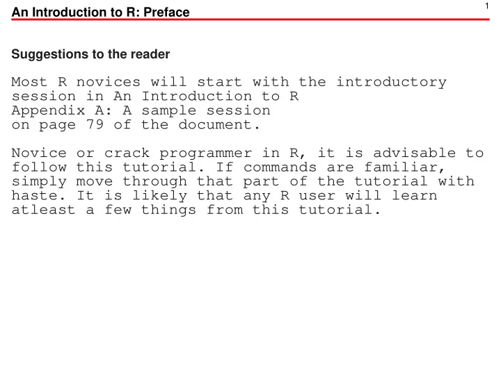
1

An Introduction to R: Preface Suggestions to the reader

Most R novices will start with the introductory session in An Introduction to R Appendix A: A sample session

• n page 79 of the document.

Novice or crack programmer in R, it is advisable to follow this tutorial. If commands are familiar, simply move through that part of the tutorial with

• haste. It is likely that any R user will learn

atleast a few things from this tutorial.

2

1.4 R and the window system; 1.5 Using R interactively

Provided the popularity of the Windows Operating System (OS) generally and its use on the desktops in the labratory for STAT 695V, what is common interactivity in the UNIX environment should also be understood for the use in the R GUI Windows platform. There is an h: drive on your ITaP account. Access it. To make a ’subdirectory’ (folder) called "work" in it, right click in an open space, scroll down to "New", select "Folder", and name it "work". Once this is done, in R observe the following commands: > getwd() [1] "h:/..." > setwd("h:/work") > getwd() [1] "h:/work" You will need to do this EVERY time you open up R unless you establish setwd("h:/work") as a command in your .First function (p. 48) within your ".Rprofile" file, which is initiated upon opening R. However, this practice is not recommended even if you establish a most commonly used directory. Thus, just start every R session in this way.

3

1.5 Using R interactively...Purpose

For a task of any size, files from a R session will almost inevitably need to be created. Once determining the best location for files for the task to be undertaken. When you determine this for the project at hand you will want to create the necessary directory and set the Working Directory (WD) to it immediately proceeding the initiaititiation of your R session. Do this now for this class.

4

1.10 Executing commands from or diverting output to a file

A test file called "lecture1.R" to observe how section 1.10 works has been created in the R data files subdirectory. The file loads the Permanent Seat Licenses (PSLs) Data Frame (DF), which will be a running example for these slides. Save it to your WD for this class then input the following commands: > source("lecture1.R") > ls() [1] "psl.rawsold.df" > head(psl.rawsold.df) day month year num area sec row total perseat price 28 8 2007 4 265sc3 304 10 20000 5000 265 > attach(psl.rawsold.df) #To be run with data of use. > save(perseat, file = "psl.rawsold.response.RData") > q() Reopen R and input these commands: > load("psl.rawsold.response.RData") > ls() [1] "perseat" > head(perseat) [1] 5000 4950 11000 5500 16500 6125

5

2 Simple manipulations; numbers and vectors: 2.1 Vectors and assignment

R is based on a vectorization system, so numbers are merely vectors of length 1. There are multiple ways

• f assigning an object of class number:

x <- 1 == x <- c(1) == c(1) -> x == 1 -> x == assign("x", 1) == assign("x", c(1)) Similarly for vectors of length = n > 1 aside from the fact that the function c() (concatenate) must be used for vectors of length(x) = n > 1: x <- c(1, 2) == c(1, 2) -> x == assign("x", c(1, 2)) In most cases the "=" operator will suffice for "<-", but you may as well utilize the pointer convention to avoid times when the alternative will not work.

6

2.2 Vector arithmetic

The elementary arithematic operators of +, -, *, /, ˆ are operable on vectors in R as well as other common functions of log, exp, sin, cos, tan, sqrt, max, min, range, sum, prod, length, floor, ceiling, round, sort, mean(x) == sum(x)/length(x), median, fivenum, summary, var(x) == sum((x - mean(x))ˆ2)/(length(x) - 1) == sˆ2 A few examples of these operators are in use below: > load("psl.rawsold.response.RData") > head(log(perseat, base = 2)) [1] 12.28771 12.27321 13.42522 12.42522 14.01018 12.5 > sum(perseat) [1] 7805644 > length(perseat) [1] 988 > summary(perseat)

• Min. 1st Qu.

Median Mean 3rd Qu. Max. 300 4250 6250 7900 10000 46250 > sd(perseat) [1] 6239.572

7

2.3 Generating regular sequences

seq, rep, and ":" are vector operators more specific than c() that reduce the amount of time it takes to program vectors of regular sequences. For a < b: a:b == c(a, a + 1,..., a + i) where b - 1 < a + i <= seq(a, b, by = 1) == a:b rep(a, b) == rep(a, floor(b)) == c(a, a,...,a) (b as) rep(c(a, b), each = b) == c(rep(a, b), rep(b, b)) d*a:b == c(d*a, d*(a + 1),..., d*(a + i)) where d*(b - 1) < d*(a + i) < d*b seq(a, b, d) == c(a, a + d,..., a + d*j) where b - d < a + d*j <= b seq(length = n, from = a, by = d) == c(a, a + d,...) For a > b the sequences are merely reversed in order. An example of these operators is in use below: > 3*1.5:9.75 [1] 4.5 7.5 10.5 13.5 16.5 19.5 22.5 25.5 28.5

8

2.4 Logical vectors

The logical operators of <, <=, >, >=, !, |, &, == determine the logical condition of TRUE, FALSE, | NA

• n vectors at each index. Logical vectors may be

used in ordinary arithmetic, in which case they are coerced into numeric vectors of FALSE == 0, TRUE == 1. A few examples of these operators are in use below: > load("psl.rawsold.perseat.RData") > bin <- perseat > 5500 & perseat < 16500 > head(bin) [1] FALSE FALSE TRUE FALSE FALSE TRUE > bin01 <- as.numeric(bin) > bin01 [1] 0 0 1 0 0 1

9

2.5 Missing values

NA is used for "Not Available" missing and NaN is used for "Not a Number" and the functions of is.na() to yield true for either NAs or NaNs and is.nan() to yield true for only NaNs A few examples of these operations are in use below: > x <- c(1, NA, 4, 0/0) > x [1] 1 NA 4 NaN > is.na(x) [1] FALSE TRUE FALSE TRUE > is.nan(x) [1] FALSE FALSE FALSE TRUE

10

3.4 The class of an object

All objects in R have a class, reported by the function class. For simple vectors this is just the mode, for example "numeric", "logical", "character",

• r "list", but "matrix", "array", "factor", and

"data.frame" are other possible values.

11

4 Ordered and unordered factors

A factor is a vector object used to specify a discrete classification (grouping) of the components

• f other vectors of the same length. R provides both
• rdered and unordered factors. While the "real"

application of factors is with model formulae, we here look at a specific example.

12

4.1 Permanent Seat Licenses (PSLs) example

The PSL data file is in the R data files subdirectory. Save it to your WD for this class then input the following commands: > load("psl.rawsold.RData") > attach(psl.rawsold.df) > head(area) [1] 265sc3 335mc3 265sc2 265sc2 335mc2 110s3 13 Levels: 90e2 108a1 110s3 120m3 125p3a2 ... 385pc23 > class(area) [1] "factor" > levels(area) [1] "108a1" "110s3" "120m3" "125p3a2" "128s1" ...

13

4.2 The function tapply() and ragged arrays

tapply(numeric, factor, function) stands for table apply, which in a tabular fashion extends/applies a function that can be applied to a numeric vector to be separated via a factor vector of the same data frame of the same vector length. This is an extraordinarilly useful function to receive quick statistical summaries per the factor(s) of the data frame to be analyzed. As examples, take the 5-# + mean, summary(perseat) and sort(median(perseat)) conditioned on (per) area: > load("psl.rawsold.RData") > attach(psl.rawsold.df) > tapply(perseat, area, summary) $’108a1’

• Min. 1st Qu.

Median Mean 3rd Qu. Max. 5667 7250 8075 8268 9250 13750 $’110s3’ ... > sort(tapply(perseat, area, median)) 265sc3 265sc2 335mc3 90e2 110s3 125p3a2 ... 2250.00 4250.00 4975.00 5162.5 7000.00 7875.0 ...

14

4.3 Ordered Factors

The levels of factors are stored in alphabetical

• rder, or in the order they were specified to factor

if they were specified explicitly. Thus, typically, it is left to the analyst to alter the order of the levels of a factor manually if one should exist in the factor. This will aid in the comprehension of your analysis particularly when plotting utilizing lattice graphics. The levels of area in the PSL Data Frame (DF) are not ordered in the preferred order. A more logical and useful ordering would be to order them by price. It is nearly there by virtue of the applied alphabetical ordering already in place, so the necessary adjustment will be minimal: > load("psl.rawsold.RData") > attach(psl.rawsold.df) > n <- length(levels(area)) > area <- factor(area, levels(area)[c(n, 1:(n - 1))]) > psl.rawsold.df$area <- area > save(psl.rawsold.df, file = "psl.rawsold.RData") > levels(area) [1] "90e2" "108a1" "110s3" "120m3" "125p3a2" ...

15

5.1 Arrays; 5.9 The concatenation function, c() with arrays

Vectors are 1-dimensionsal (1-dim or 1-d), matrices are 2-dim, and arrays are k-dim for k \in N. Arrays will be output in lieu of vectors or matrices when they are to be categorized via a factor such as in the use of the tapply() function. > load("psl.rawsold.RData") > attach(psl.rawsold.df) > class(tapply(perseat, area, median)) [1] "array" > dim(tapply(perseat, area, median)) [1] 13 > names(tapply(perseat, area, median)) [1] "90e2" "108a1" "110s3" "120me" "125p3a2" ... > c(tapply(perseat, area, median)) 90e2 108a1 110s3 120m3 125p3a2 128s1 .. 5162.5 8075.00 7000.00 12500.00 7875.00 10750.0 .. > class(c(tapply(perseat, area, median))) [1] "numeric" > as.vector(tapply(perseat, area, median)) [1] 5162.5 8075.0 7000.0 12500.0 7875.0 10750.0 .. > class(as.vector(tapply(perseat, area, median))) [1] "numeric"

16

5.10 Frequency tables from factors

Although frequency tables can be constructed via the tapply(interaction(factor A, factor B,...), interaction(factor A, factor B,...), length) the more apparent function is to know that you desire a frequency table and simply utilize the function table(factor A, factor B,...) Let’s see this with the PSL data frame: > load("psl.rawsold.RData") > attach(psl.rawsold.df) > table(area) 90e2 108a1 110s3 120m3 125p3a2 128s1 ... 240 74 41 19 34 70 ... > tapply(area, area, length) 90e2 108a1 110s3 120m3 125p3a2 128s1 ... 240 74 41 19 34 70 ... > table(area, num) num area 1 2 3 4 5 6 7 8 10 90e2 14 149 8 56 9 1 2 1 ...

17

6.3.2 attach() and detach(); 6.3 Data frames

The command attach() has been peppered throughout these slides to make utilization of the PSL examples work smoother. For one data frame at a time, the vectors of that data frame can then be cited simply with the names of the vectors themselves as oppose to having to utilize the entire root command, which is extraordinarily useful in reducing the length of commands to be run through the R console. Thus, once attach(psl.rawsold.df) is issued as a command, to access psl.rawsold.df$perseat is as easy as utilizing "perseat" the vector. However, keep in mind, manipulations now made to the vector perseat will not affect the data frame in the column perseat

• f psl.rawsold.df$perseat. This itself can also be

useful to test manipulations without accidentally changing your main data frame from its original form and possibly losing the correct data. Be sure to read section 6.3 (p. 27-29) very carefully as it does provide the best and most effective way to work with data for simplicity and security in R.

18

7 Reading data from files

There are multiple different commands to import data from varying files depending on the type of file the data abides.

• 1. read.table() is for .txt or text files
• 2. read.csv() is for .csv files, which is a ”save as” option for Excel files
• 3. scan() will read in .dat or .data file
• 4. load() will read in .RData files, which can be dfs, lists, or other forms
• 5. data() will access a data set from a built in package

Some examples are in the R folder and can be run on your end: > psl.rawsell.df <- read.table("psl.txt") > psl.rawsold.csv.df <- read.csv("psl.csv") > psl.rawsold.RData.df <- load("psl.rawsold.RData") > data(package = "lattice") #If not already installed > library(lattice) #To be run at initiation of R > data(singer, package = "lattice")

19

7.4 Editing data

For minor adjustments to a data frame or a matrix of a manageable size, maybe say n < 100 & p < 20, edit can be a useful call in R. It brings up your object in a spreadsheet so that you can go to specific entries via visual inspection as oppose to demanding that you know the locations via coordinates of the values that require a swap. You can navigate the usefulness of this option for yourself: > load("psl.rawsold.RData") > edit(psl.rawsold.df) > # Have at!

20

8.1 R as a set of statistical tables Distribution R name additional arguments beta beta shape1, shape2, ncp binomial binom size, prob Cauchy cauchy location, scale chi-squared chisq df, ncp exponential exp rate F f df1, df2, ncp gamma gamma shape, scale geometric geom prob hypergeometric hyper m, n, k log-normal lnorm meanlog, sdlog logistic logis location, scale negative binomial nbinom size, prob normal norm mean, sd Poisson pois lambda signed rank signrank n Student’s t t df, ncp uniform unif min, max Weibull weibull shape, scale Wilcoxon wilcox m, n

21

8.2 Examining the distribution of a set of data; Lattice graphics introduced

It is this section that initiates graphics to aid in the determination of the distributional properties of a data set. Graphics and plots are at the core of determining the distributional properties of a data set and lattice graphics is the best computer program graphics package available to run this critical and initial part of a statistical analysis for its plyability, flexibility, ease in use, and well

• rganized open source library (as well as R in

general) to utilize all of its effective input

• ptions beyond default settings.

This section initiates its plotting analysis of the response variable with a histogram. However, the first plot to be observed for any data set should be a qqnorm plot of the response variable. The code to do this for the PSL data is on the next slide with the plot on the slide after the slide of the code.

22

qqnorm of perseat code

> library(lattice) > load("psl.rawsold.RData") > attach(psl.rawsold.df) > trellis.device(pdf, file = "perseat.qqmath.pdf") > qqmath(˜perseat, data = psl.rawsold.df, main = "qqnorm Plot of perseat (units = $)", panel = function(x) { panel.qqmath(x, pch = ".", cex = 1.5) panel.qqmathline(x) }) > dev.off()

23

qqnorm of perseat plot

qqnorm Plot of perseat (units = $)

qnorm perseat

10000 20000 30000 40000 −2 2

24

Observations from qqnorm of perseat plot and more formal tests of normality

Points appear to roughly follow an exponential pattern, so perseat does not appear normal. However, to confirm this hypothesis, more formal tests of normality such as the Shapiro-Wilk test and the Kolmogorov-Smirnov test should be employed to assert this claim. Upon such evidence, the exponential pattern indicates a need for a transformation, most likely logarithmic. A boxcox plot to further evidence the optimal transformation will be needed after the normality tests. The plot will be placed on the next slide while the code necessary to run the tests of normality and make the plot are below: > library(MASS) > load("psl.rawsold.RData") > attach(psl.rawsold.df) > shapiro.test(perseat) > ks.test((perseat-mean(perseat))/sd(perseat), pnorm) > trellis.device(pdf, file = "perseat.boxcox.pdf") > boxcox(perseat ˜ 1, ylab = "logLikelihood perseat") > dev.off()

25

boxcox of perseat plot

−2 −1 1 2 −5500 −5000 −4500 −4000 −3500 λ logLikelihood perseat 95%

26

Observations from boxcox of perseat plot

With transformations, simplicity and comprehension are the top priorities. This means λ = 1, 0, 2, −1, 1/2, ... are the best in order. Of course, this ordering of priority cannot be taken so strictly as to completely

• ver look the log-likelihood confidence interval. In
• ur case, the confidence interval nearly centers

(maximum of log-likelihood/optimal) over λ = 0, so is optimum. This implies the simplest, most comprehendabe, and most likely transformation is logarithmic as was evidenced in the qqnorm plot. Thus, for the best scale and human comprehension, a log(perseat, base = 2) transformation should be used. Further, once this transformation is undertaken, again a qqplot of the transformed data should be

• bserved, which is done on the next slide.

27

qqnorm of log2perseat plot

qqnorm Plot of log2perseat (units = log2$)

qnorm log2perseat

8 10 12 14 −2 2

28

Observations from qqnorm of log2perseat plot

Even the transformed response variable does not appear normal while such suspicions can be confirmed with the same tests of normality from above. However, this is common in real world data and is not a problem provided we possess covariates in the PSL data set that the response can be modeled upon. This further analysis will be delayed for the moment for later slides as it no longer follows the goal of 8.2.

29

9.2.2 Repetitive execution: for loops, repeat and while Warning:

for() loops are used in R code much less often than in compiled languages. Code that takes a ’whole

• bject’ view is likely to be both clearer and faster

in R. Other looping facilities include the > repeat expr statement and the > while (condition) expr while() is often a more effective looping condition when the looping procedure more fluidly derives from a logical as oppose to a numeric length vector.

30

10 Writing your own functions; 10.1 PSL example

There are a many built in functions in R, which cover a majority of the demands of R users. However, from time to time, every R user requires a little more flexibility than what the built in functions provide

• n their own. Typcally, all this will require on the

part of an R user is "wrap around" functions. A couple of "wrap around" functions utilized for the PSL data set are coded below: > load("psl.rawsold.RData") > attach(psl.rawsold.df) > myshapiro.test <- function(x) shapiro.test(x)$p > tapply(log2perseat, area, myshapiro.test) 90e2 108a1 110s3 120m3 .. 6.155058e-05 3.145007e-01 5.440043e-02 6.661643e-02 .. > myks.test <- function(x) ks.test((x - mean(x))/sd(x), pnorm)$p > tapply(log2perseat, area, myks.test) 90e2 108a1 110s3 120m3 125p3a2 0.01901863 0.81850326 0.46403603 0.94613687 0.18501850

31

10.3 Named arguments and defaults

Most functions in R, as well as functions you can write on your own, already possess inputted values. These defaults are alterable for the flexibility of the user, but exist for there is a definitively most demanded use of the input, such as the statistical tables, and where users have not even thought of all the potential inputs, such as graphics commands. For instance, lattice graphics function commands possess a plethora of input options that many users are even unaware of their existence. Provided the depth of help files on functions this is something that can easily be remedied with a little diligence, but often times this is not necessary where the defaults are quite effective.

32

10.8 Customizing the environment

Within your .Rprofile file there are the functions of:

• 1. .First(), which will run automatically as you open R. The purpose of this function

is for users that begin to recognize commands they run at the beginning of each R session as part of their personal set up to have R automatically do it for them to save time at the beginning of each R session.

• 2. .Last(), which will run automatically upon quitting R. The purpose of this function

is to avoid accidentally quitting R before saving objects that you do not want to lose.

A potential initial .Rprofile function for you: .First <- function() { library(lattice) #You want this loaded every time. library(MASS) #You want this loaded too. } .First() .Last <- function() { graphics.off() #A small safety measure to have setwd("h:/previousRsession") #Create directory 1st save(ls(), file = "pws.RData") #Same as graphics } .Last()

33

12 Graphical procedures

Chapter 12: Graphical procedures should preempt Chapter 11: Statistical models in R, because before choosing models to fit real world data sets some semblence of the structure of the response variable(s) and how the potential explanatory variable(s) are relating to the response must be

• bserved through plotting and basic human pattern
• detection. Without this step, nothing but crude in

the dark guessing as to the true nature of the relationships of the variable(s) is available. Thus, marginal plot(s) of the response variable(s), then in comparison to potential explanatory variable(s), and finally conditioned via trellis display over factor

• r factor induced numeric explanatory variable(s)

must be run before testing potential linear models. This is a time consuming process, but is the first in a proper data analysis. Once some semblence of a regression structure has been determined via plotting, then statistical models can be procured in R for the purpose of model determination where more

• bjective and less diagnostic measures can also be

utilized to support hypotheses.

34

Lattice graphics continued with the PSL data frame

Thus far in the PSL data frame analysis we have only transformed the singular response variable. However, the only value to performing such a transformation is for the purposes of fitting a model regression to our

• response. Thus, the next step is to determine the

potential explanatory variable(s) that could impact the perseat value for a PSL and then to look at marginal plot(s) of log2perseat with those potential explanatory variable(s) and eventually the trellis

• displays. The potential explanatory variable(s) are:
• 1. area within Soldier Stadium the seats abide
• 2. price for a single day ticket of a seat within a particular area
• 3. row within a given section and area
• 4. date of transaction
• 5. section the seats abide
• 6. number or seats sold
• 7. Reconfigurations of the provided data from the variables above

35

bwplot() of log2perseat conditioned on area choice and code

Since area is likely to possess the greatest impact

• n perseat PSL prices that is the first potential

explanatory variable we wish to plot log2perseat

• against. The potential choices are bwplot() and

qqmath(). Since our goal is one of determining the regression relationship, bwplot() should be utilized, to compare the distributional properties of log2perseat per each area against one another in the most apparent and simple way possible where qqmath() would make it difficult to do this in one plot. > library(lattice) > load("psl.rawsold.RData") > trellis.device(pdf, file = "log2perseatvsarea.bwplot.pdf") > bwplot(area ˜ log2perseat, data = psl.rawsold.df, xlab = "log2perseat (units = log2$)", ylab = "area", main = "Box Plot of log2perseat by area") > dev.off()

36

bwplot() of log2perseat conditioned on area plot

Box Plot of log2perseat (units = log2$) by area

log2perseat (units = log2$) area

90e2 108a1 110s3 120m3 125p3a2 128s1 135m1 135ms2 265sc2 265sc3 335mc2 335mc3 385pc23 8 10 12 14

37

Observations from bwplot() of log2perseat conditioned on area plot

With the factor of area ordered by the single day ticket price, it can be observed that once the single day ticket price dramatically jumps from $135 to $265 in the club area the variability increases vastly, there is heavy left tail or skew to the left, and the medians are typically smaller. Thus, on the whole, the club seats PSLs sell for less, which from the nature of the ordering on the factor appears to be likely due to the immense proportional jump in the single day ticket price from other tickets. However, this plot still does not provide any substantial guidance in determining a good model for

• ur data set.

38

xyplot() of log2perseat vs. row choice and code

Now we will look at the potential quantitative explanatory variable of row on log2perseat. Now that both response and explanatory variable will be quantitative we can observe its marginal affect via an xyplot(). > library(lattice) > load("psl.rawsold.RData") > trellis.device(pdf, file = "log2perseatvsrow.xyplot.pdf") > xyplot(log2perseat ˜ row, data = psl.rawsold.df, xlab = "row", ylab = "log2perseat (units = log2$)", main = "log2perseat vs. row", skip = c(rep(FALSE, 8), rep(TRUE, 2)), aspect = 1.5, panel = function(x, y) { panel.points(x, y, pch = ".", col = 1, cex = 1.5) panel.loess(x, y, span = 1, family = "gaussian") panel.lmline(x, y) }) > dev.off()

39

xyplot() of log2perseat vs. row plot

log2perseat vs. row

row log2perseat (units = log2$)

8 10 12 14 5 10 15 20 25

40

Observations from xyplot() of log2perseat vs. row plot

A negative, essentially linear relationship, but with what appears to be great variability indicates that the strength of the linear relationship is weak to moderate at best without even running the lm() command in R and determining the effectiveness of the

• model. Either way, we know the marginal impact of row
• n log2perseat, even if it demands that we must keep

digging.

41

xyplot() of log2perseat vs. row conditioned on area choice and code

Knowing now the general marginal affect due to area and row independently, what is the impact of row per any given area? Is it similar or nearly the same per area or does it vary greatly similar to the box plots for log2perseat conditioned on area? Thus, the final plot to be portrayed in this part of the rintro slides is to see the last main plotting mechanism of conditioning on a factor variable. There are still more potential explanatory varables to explore, so the graphics analysis is not through. However, this should lend you the code and general direction from which to progress a graphical analysis of a data set. > xyplot(log2perseat ˜ row | area, data = psl.rawsold.df, xlab = "row", ylab = "log2perseat (units = log2$)", main = "log2perseat vs. row by area", skip = c(rep(FALSE, 8), rep(TRUE, 2)), panel = function(x, y) { panel.points(x, y, pch = ".", col = 1, cex = 1.5) panel.loess(x, y, span = 1, family = "gaussian") panel.lmline(x, y)})

42

xyplot() of log2perseat vs. row conditioned on area plot

log2perseat vs. row by area

row log2perseat (units = log2$)

8 10 12 14 5 10 15 20 25

90e2 108a1

5 10 15 20 25

110s3 120m3

5 10 15 20 25

125p3a2 128s1 135m1 135ms2

8 10 12 14

265sc2

5 10 15 20 25

265sc3 335mc2

5 10 15 20 25

335mc3 385pc23

43

Observations from xyplot() of log2perseat vs. row conditioned on area plot

As was mentioned with the bwplot(), there appears to be greater variability in the club areas. Thus, regressing on row has not made a significantly greater impact on those sections. However, the decrease in perseat price as row increases does still appear greater in the club sections even if the variability has not reduced. This is potentially a decent place to begin model testing. However, even as lm() models are run, trellis displays will still be necessary to assert that the residuals do not abide by a pattern against any of the other potential explanatory variable(s).

44

11.2 Linear models

The first model to be assessed based on the graphical analysis of the PSL data is that of log2perseat regressed on the interaction of area and row. > load("psl.rawsold.RData") > attach(psl.rawsold.df) > mod1 <- lm(log2perseat ˜ area + area:row - 1, data = psl.rawsold.df) > summary(mod1) > mod1a <- lm(log2perseat ˜ area*row, data = psl.rawsold.df) > summary(mod1a) The models are identical except in interpretation and in the validity of the statistics. mod1 possesses the more valuable interpretation, while mod1a possesses the valid statistics as it demonstrates the affect of changing from one area to another as oppose to suggesting that each area is significantly different from no affect. Thus, the Multiple R-squared: 0.6681 shows that 66.81% of the variation in log2perseat can be explained by the regression on area*row and which coefficients are truly significantly different.

45

11.3 Generic functions for extracting model information

The value of lm() is a fitted model object; technically a list of results of class "lm". Information about the fitted model can then be displayed, extracted, plotted and so on by using generic functions that orient themselves to objects

• f class "lm". These include:

add1 deviance formula predict step alias drop1 kappa print summary anova effects labels proj vcov coef family plot residuals

In the previous slide I utilized summary(), which is also applicable for the numeric class with a different output. It provides a 5-# summary on residuals(), coef(), as well as other useful statistics, so is a good start in evaluating the quality of the model. deviance() outputs the Residual sum of squares, weighted if appropriate, a quick simple numeric summary for model comparison purposes. plot() will quickly provide a couple useful plots for evaluating your model in a diagnostic manner, even if you should make better plots for diagnostics.

46

Better diagnostics with lattice graphics

Since mod1 from our PSL data set splits over the factor of area, the diagnostic plots utilized to assess the quality of the model should also be split

• ver area with trellis display plots. Since we have

still yet to utilize other potential quantitative explanatory variable(s), we can utilize at least one

• f them to observe the residuals as they change over
• ne or more of those variables. Since section number

in its current state is not structured as a quantitative let alone ordinal scale categorical variable, number of seats sold possesses too few number of observations at 5 or more (> table(num)), price is already essentially incorporated in area, it leaves date. Date is most capably utilized by extracting only the year information for a large enough sample size for each year. Thus, the plot of choice for these slides is given below.

47

xyplot() of resmod1 vs. year conditioned on area code

> library(lattice) > load("psl.rawsold.RData") > attach(psl.rawsold.df) > mod1 <- lm(log2perseat ˜ area + area:row - 1, data = psl.rawsold.df) > save(mod1, file = "lmmod1.RData") > psl.rawsold.df$resmod1 <- resid(mod1) > attach(psl.rawsold.df) > save(psl.rawsold.df, file = "psl.rawsold.RData") > trellis.device(pdf, file = "resmod1vsyearbyarea.xyplot.pdf") > xyplot(resmod1 ˜ year | area, data = psl.rawsold.df, xlab = "year", ylab = "resmod1 (units = log2$)", main = "resmod1 vs. year by area", panel = function(x, y) { panel.points(x, y, pch = ".", col = 1, cex = 1.5) panel.loess(x, y, span = 1, family = "gaussian") panel.lmline(x, y) })

48

xyplot() of resmod1 vs. year conditioned on area plot

resmod1 vs. year by area

year resmod1 (units = log2$)

−3 −2 −1 1 2 2007 2009 2011 2013

90e2 108a1

2007 2009 2011 2013

110s3 120m3

2007 2009 2011 2013

125p3a2 128s1 135m1 135ms2

−3 −2 −1 1 2

265sc2

2007 2009 2011 2013

265sc3 335mc2

2007 2009 2011 2013

335mc3 385pc23

49

11.5 Updating fitted models...what we are going to do instead...backfitting

The update() function is largely a convenience function that allows a model to fitted that differs from one previously fitted usually by just a few additional or removed terms. Its form is > new.model <- update(old.model, new.formula) Thus, although you may find this function along with add1(), drop1(), and step() along with the ’.’

• perator within all of these functions and lm()

useful, they are by no means necessary. What is necessary though is the concept of back

• fitting. From the previous slide’s plot, it is
• bservable that there is essentially no affect from

the variable year for the non-club areas while in the club areas there appears to be a very similar negative linear relationship between the resmod1 and

• year. Incorporating this requires the knowledge of

and application of the concept of back fitting, which is to say we will fit a lm() of resmod1 vs. year for

• nly the subset of club areas.

50

Code for plotting to evaluate the effectiveness of mod2

> load("psl.rawsold.RData") > attach(psl.rawsold.df) > mod2 <- lm(resmod1 ˜ I(year - 2006), data = psl.rawsold.df, subset = price > 135) > save(mod2, file = "lmmod2.RData") > psl.rawsold.df$Iareaisclub <- as.numeric(price > 135 > resmod2 <- resmod1 - Iareaisclub*coef(mod2)[1] - Iareaisclub*coef(mod2)[2]*(year - 2006) > psl.rawsold.df$resmod2 <- resmod2 > save(psl.rawsold.df, file = "psl.rawsold.RData") > trellis.device(pdf, file = "resmod2byareaclubtop.qqmath.pdf") > qqmath(˜resmod2 | area, data = psl.rawsold.df, main = "qqnorm Plot of resmod2 (units = log2$)", layout = c(5, 3), skip = c(rep(FALSE, 8), rep(TRUE, 2)), panel = function(x) { panel.qqmath(x, pch = ".", cex = 1.5) panel.qqmathline(x) }) > dev.off()

51

qqmath() of resmod2 conditioned on area plot

qqnorm Plot of resmod2 (units = log2$)

qnorm resmod2

−2 −1 1 2 −3 −2 −1 1 2 3

90e2 108a1

−3 −2 −1 1 2 3

110s3 120m3

−3 −2 −1 1 2 3

125p3a2 128s1 135m1 135ms2

−2 −1 1 2

265sc2

−3 −2 −1 1 2 3

265sc3 335mc2

−3 −2 −1 1 2 3

335mc3 385pc23

52

Observations from qqmath() of resmod2 conditioned on area plot; dotplot() of resmod2 Standard Deviations (SDs) conditioned on area code

The residuals all seem normal enough within their respective areas, but the variabilities within each area appear dramatically different. Thus, the model needs to incorporate SDs conditioned on area. To

• bserve these different SDs we again utilize the

tapply() function, the Cleveland dotplot(), and follow through with hypotheses tests of equality of variances. > sort(tapply(resmod2, area, sd)) 108a1 110s3 135ms2 120m3 90e2 ... 0.2646775 0.3301854 0.3452735 0.3752475 0.3832580 ... > dotplot(tapply(log2perseat, area, sd), data = psl.rawsold.df, main = "Standard Deviations (SDs) of resmod2 by area", xlab = "Standard Deviation (SD) of resmod2", ylab = "area") > bartlett.test(resmod2 ˜ area, data = psl.rawsold.df) [1] 7.143686e-47

53

dotplot() of resmod2 standard deviations conditioned on area plot

Standard Deviation of resmod2 by area

Standard Deviation (sd) of resmod2 area

90e2 108a1 110s3 120m3 125p3a2 128s1 135m1 135ms2 265sc2 265sc3 335mc2 335mc3 385pc23 0.4 0.6 0.8

54

Observations from dotplot() of resmod2 SDs conditioned on area plot

The SDs are obviously statistically different based

• n Bartlett’s Test and tapply() is sufficient to

assess how, but the dotplot() is more effective. All along we have been distinguishing differences between the club areas and non-club areas and this case appears to be no different. At bare minimum, the SDs from the club areas are of a distinguishably different population than the SD from the non-club

• areas. However, once within these subpopulations do

the SDs vary? This investigation is left to you as we move back to "An Introduction to R".

55

11.6.1 Families; 11.6.2 The glm() function, The gaussian family; 11.6 glm Family name Link functions binomial logit, probit, log, cloglog gaussian identity, log, inverse Gamma identity, inverse, log inverse.gaussian 1/mu2, identity, inverse, log poisson identity, log, sqrt quasi logit, probit, cloglog, identity, inverse, log, 1/mu2, sqrt

A call such as > mod1 <- glm(log2perseat ˜ area + area:row - 1, family = gaussian, data = psl.rawsold.df) achieves the same result as > mod1 <- lm(log2perseat ˜ area + area:row - 1, data = psl.rawsold.df) but much less efficiently. GLM is a development of LM to accomodate both non-normal response distributions and transformations to linearity in a clean and straightforward way. Typically, we recommend you perform tranformations

• ne step at a time with lattice graphics to assure a

better analysis.

56

rintro view graphs conclusion

These rintro view graphs are merely a synopsis of an

• ver 100 page set of notes summary/tutorial into the

use of the R language. Thus, you should not interpret these view graphs as the be all holy grail to the use

• f the R language. However, hopefully through the

process of going through these view graphs, the coding between, with a fresh outlook on a currently relavent data set that utilizes the very essential lattice graphics package you have built a familiarity that will allow you to initiate your own data

• analyses. As you embark on this process yourself you

should keep these view graphs, An Introduction to R, and as many of its references, listed on the next slide, as close at hand as possible. Good luck!

57

Appendix F References

• D. M. Bates and D. G. Watts (1988), Nonlinear Regression Analysis and Its
• Applications. John Wiley & Sons, New York.

Richard A. Becker, John M. Chambers and Allan R. Wilks (1988), The New S

• Language. Chapman & Hall, New York. This book is often called the ”Blue Book”.

John M. Chambers and Trevor J. Hastie eds. (1992), Statistical Models in S. Chapman & Hall, New York. This is also called the ”White Book”. John M. Chambers (1998) Programming with Data. Springer, New York. This is also called the ”Green Book”.

• A. C. Davison and D. V. Hinkley (1997), Bootstrap Methods and Their Applications,

Cambridge University Press. Annette J. Dobson (1990), An Introduction to Generalized Linear Models, Chapman and Hall, London. Peter McCullagh and John A. Nelder (1989), Gerneralized Linear Models. Second edition, Chapman and Hall, London. John A. Rice (1995), Mathematical Statistics and Data Analysis. Second edition. Duxbury Press, Belmont, CA.

• S. D. Silvey (1970), Statistical Inference. Penguin, London.