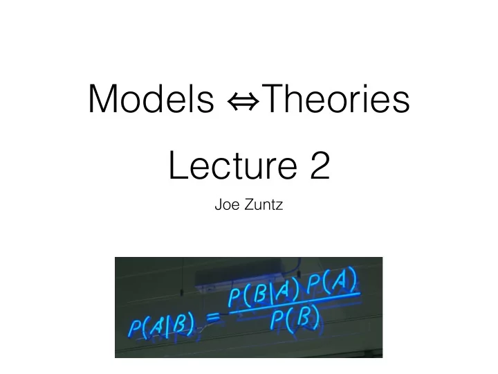
Models Theories Lecture 2 Joe Zuntz Overview Notes on Gaussians - PowerPoint PPT Presentation

Models ⇔ Theories Lecture 2 Joe Zuntz

Overview • Notes on Gaussians • Type 1A Supernova Likelihoods (data • Building Priors modelling) • Building Likelihoods • What is perturbation theory • Distance measures in cosmology • Weak Lensing Likelihoods (handling • Cepheid Likelihoods systematic errors) (fitting a straight line)

Notes on Gaussians

Gaussians: 
 Properties • Central limit theorem: 
 Given a collection of random variables X i : n 1 X � ( X i − µ i ) → N (0 , 1) s n i =1 � n X s 2 σ 2 n = i � i =1 • Provided that: 1 X ( X − µ i ) 2 ⇤ ⇥ → 0 E s 2 n

Gaussians: 
 Properties • Central limit theorem: Single 
 Mean of 2 distribution Mean of 3 Mean of 4

Gaussians: 
 Multivariate  � 1 − 1 2( x − µ ) T C − 1 ( x − µ ) P ( x ; µ , C ) = 2 | C | exp n (2 π ) • C is the covariance matrix - describes correlations between quantities • For example: data points often have correlated errors

Descriptive Statistics: Covariance σ XY > 0 σ XY < 0 Y Y X X

Building Likelihoods: 
 General Rules • Most of this is physics! • When you don’t know something, marginalize over it • Reduce to probabilities you do know • Use the problem logic to understand things • What quantities are independent? • Basic distributions like Poisson, Gaussian, etc., very useful

Building Priors • Priors encode what you knew about the parameters before you got this new data • Results of previous experiments! • Physical limits (e.g. positivity) • Experiment to check dependence of answers • If changing your prior changes the results significantly then new data not very informative

Building Priors • Lazy: just use flat priors on things • Remember how probabilities transform: u = f ( x ) P ( u ) = P ( x ) /f 0 ( x )

Data Sets, Likelihoods, and Limitations • Cosmic Microwave • Cepheid Variables � Background � • Type IA Supernovae � • Redshift Space Distortions � • Baryon Acoustic • Weak Lensing � Oscillations � • Large-Scale Structure � • Strong Lensing � • Cluster Counts � • Light element abundances � • 21cm line structure � • Globular cluster ages � • Lyman Alpha Forest

Data Sets, Likelihoods, and Limitations • Cosmic Microwave • Cepheid Variables � Background • Type IA Supernovae • Redshift Space Distortions • Baryon Acoustic 
 • Weak Lensing Oscillations • Large-Scale Structure • Strong Lensing • Cluster Counts • Light element abundances • 21cm line structure • Globular cluster ages • Lyman Alpha Forest

Distance Measures in Cosmology Different distance measures depending on exactly what you measure. See Hogg (2000).

Co-moving LOS Distance • Co-moving line of sight distance describes integral of distances scaled to the cosmic expansion Z z d z 0 D c ( z ) = H ( z 0 ) 0 Ω M (1 + z ) 3 + Ω k (1 + z ) 2 + Ω Λ p H ( z ) = H 0

Co-moving Transverse Distance • Co-moving transverse distance accounts for the curvature of space: ! c c D M = sin k D c p p | Ω k | | Ω k | H 0 H 0 8 sin x x > 0 < x = 0 sin k ( x ) = x sinh x x < 0 :

Luminosity Distance • Luminosity Distance describes relationship between flux emitted from a source and luminosity received. r L 4 π S = (1 + z ) D M D L ≡ � • Fluxes and redshifts are observable quantities: we are getting somewhere useful! • Measure D L and z of some objects 
 ⟹ constraint the H(z) and Ω values

Angular Diameter Distance • Describes relationship between angle subtended by object and object physical size � D A = ∆ x ∆ θ = D M / (1 + z ) � • If we can measure angle of object with known size then constrain expansion

Small Distances • These distances equal for close objects v = cz = H 0 D

Magnitudes • Astronomers use logarithmic system of luminosities/ distances • Apparent Magnitude m : 
 Log of observed luminosity relative to standard • Absolute Magnitude M : 
 What apparent magnitude would be if object 
 were 10 parsecs away  D L � • Distance Modulus: µ ≡ m − M = 5 log 10 − 5 1 pc

Cepheid Variables Fitting straight lines with two sources of error

Cepheid Likelihoods: 
 Model � • Linear relation between log period and magnitude • Scatter clearly not just from noise • intrinsic scatter

Cepheid Likelihoods: 
 Standard Inference • Find extragalactic Cepheids too! • Use the same linear fit to deduce their luminosity • Get redshift-distance relation H 0

Cepheid Likelihoods: 
 Model µ i = α + β log 10 [ P i / Days] V i ∼ N ( µ i , σ 2 int ) V obs ∼ N ( V i , σ 2 i ) i

Aside: Bayesian Networks β σ int α • Nice way to build/ illustrate Bayesian Networks aka P V i Hierarchical Models • Can use for inference V obs σ i i

Cepheid Likelihoods: 
 Standard Inference We want P ( p | V obs ) p ≡ { α , β , σ int } Y P ( V obs | p ) = P ( V obs | p ) i

Cepheid Likelihoods: 
 Standard Inference Z P ( V obs P ( V obs | p ) = | p V i ) P ( V i | p ) d V i i i Z P ( V obs | V i ) P ( V i | p ) d V i = i Z N ( V obs ; V i , σ 2 i ) N ( V obs ; α + β log 10 P i , σ 2 = int ) d V i i i

Building Likelihoods: 
 Example • Exercise 1 
 Show that this is given by: ✓ ( V obs − ( α + β log 10 P i )) 2 ◆ 1 P ( V obs i | p ) ∝ exp − 0 . 5 i σ 2 int + σ 2 σ 2 int + σ 2 i i • In one of the exercises you will evaluate and use this likelihood using some simulated data

H 0 Likelihoods: • Standard approach: • Use the LMC to find maximum likelihood values of the alpha, beta, and sigma parameters • Fix these parameters to analyse cosmological

H 0 Likelihoods A better way! • Simultaneously analyse LMC data and cosmological cepheids!

Exercise 2 β σ int α • Exercise 2: Extend this Bayesian Network diagram to do the simultaneous analysis P V i of LMC and extragalactic Cepheids V obs σ i i

Exercise 3 • Code up a function to calculate this likelihood

Type IA Supernovae “Standardizing” using modelling

Type IA Supernovae Physics • White Dwarf accretes matter from binary companion. • Reaches Chandrasekhar limit 1.39 M ☉ • Core becomes relativistic => equation of state changes => core cannot support mass =>supernova! • Same mass => same brightness

Type IA Supernovae Observations • Detection New image Old image Difference http://supernova.galaxyzoo.org/discoveries

Type IA Supernovae Observations • Spectroscopic follow up • redshift • type http://supernova.lbl.gov/

Type IA Supernovae Observations • Photometric follow up • Light curve http://supernova.lbl.gov/

Type IA Supernovae Observations • Standard izable Candle • Calculate luminosity from curve shape • Various empirical methods 
 SALT2: color and stretch parameters

Type IA Supernovae 
 Inference • Measure distance modulus (log luminosity) ✓ D L ◆ µ = 5 log 10 + 25 1 Mpc µ = m − M Apparent 
 Absolute 
 Magnitude Magnitude (measured) (modelled)

Type IA Supernovae 
 Inference • Need a model for the absolute magnitude given light curve shape • First, model the shape of the light curve • color and stretch

Light Curve Model c = ( B � V ) max � h B � V i M 0 ( t, λ ) = h M ( t, λ ) i M 1 ( t, λ ) = First principal component of M M ( λ , t ) = x 0 [ M 0 ( t, λ ) + x 1 M 1 ( t, λ ) + ... ] e [ cf ( λ )]

Abs Magnitude Model • Find empirically from nearby SNe with known Cepheid distance that: M i = M − α x 1 i + β c i

Type IA Supernovae 
 Inference • Nuisance parameters included in model: Measured from light curves µ = m ∗ − M 0 + α x 1 − β c Fitted nuisance parameters

Type IA Supernovae 
 Inference • So overall parameters = { Ω m , Ω Λ , H 0 , M 0 , α , β } • Steps: D theory • Theory: ( z obs ) = D L ( Ω M , Ω Λ ) L � ! D theory µ theory = 5 log 10 L + 25 1 Mpc � • “Observable”: µ obs = m ∗ obs − M 0 + α x obs − β c obs 1

Type IA Supernovae 
 Inference • Covariance = (Messy Combination of noise and nuisance params)! • Likelihood multivariate Gaussian � L ∝ | C | − 1 exp − 1 2( µ obs − µ theory ) T C − 1 ( µ obs − µ theory ) � • Caution! The priors do matter here! But by coincidence the maximum-likelihood nuisance params work okay. 
 See arxiv:1207.3705

Perturbations

Perturbations • Can probe fluctuations on top of the background mean cosmology • Need relativistic perturbation theory to predict • Will very briefly discuss extreme basics now! • Discuss codes that solve these for you, and approximations

Perturbation Theory d s 2 = a 2 � d τ 2 + d x 2 � ρ ( t ) perturb d s 2 = a 2 � − (1 + 2 Ψ )d τ 2 + (1 − 2 Φ )d x 2 � ρ ( t ) + δρ ( x , t )

Perturbation Theory • Phi and Psi are linear order perturbations to metric 
 Have similar perturbations to densities, velocities, and moments. • All quantities in Fourier space • Insert perturbed forms into Einstein and geodesic equations

Perturbation Theory Conformal Newtonian 
 Gauge