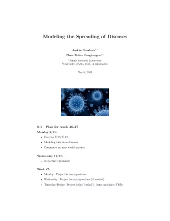
Modeling the Spreading of Diseases Joakim Sundnes 1 , 2 Hans Petter - PowerPoint PPT Presentation
Modeling the Spreading of Diseases Joakim Sundnes 1 , 2 Hans Petter Langtangen 1 , 2 Simula Research Laboratory 1 University of Oslo, Dept. of Informatics 2 Nov 6, 2018 Plan for week 45-46 Tuesday 6/11: Exer E.21, E.22 Systems of ODEs Disease
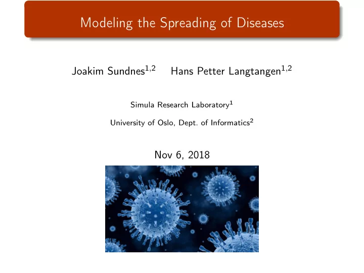
Modeling the Spreading of Diseases Joakim Sundnes 1 , 2 Hans Petter Langtangen 1 , 2 Simula Research Laboratory 1 University of Oslo, Dept. of Informatics 2 Nov 6, 2018
Plan for week 45-46 Tuesday 6/11: Exer E.21, E.22 Systems of ODEs Disease modeling Thursday 8/11: No lecture (probably) Week 46: Tuesday: Project lecture/questions (here in Sophus Lie) Thursday: No lecture Thursday/Friday: Project help ("orakel"). (time and place TBD)
We shall model a complex phenomenon by simple math (1) Plan: Use simple intuition to derive a system of difference equations to model the spread of diseases Program the difference equations in the usual way (i.e. for -loops) Explore possible model extensions See how the difference equations correspond to ordinary differential equations
We shall model a complex phenomenon by simple math (2) Assumptions: We consider a perfectly mixed population in a confined area No spatial transport, just temporal evolution We do not consider individuals, just a grand mix of them We consider very simple models, but these can be extended to full models that are used world-wide by health authorities. Typical diseases modeled are flu, measles, swine flu, HIV, ... All these slides and associated programs are available from https://github.com/hplgit/disease-modeling .
We shall model a complex phenomenon by simple math (2) Assumptions: We consider a perfectly mixed population in a confined area No spatial transport, just temporal evolution We do not consider individuals, just a grand mix of them We consider very simple models, but these can be extended to full models that are used world-wide by health authorities. Typical diseases modeled are flu, measles, swine flu, HIV, ... All these slides and associated programs are available from https://github.com/hplgit/disease-modeling .
We shall model a complex phenomenon by simple math (2) Assumptions: We consider a perfectly mixed population in a confined area No spatial transport, just temporal evolution We do not consider individuals, just a grand mix of them We consider very simple models, but these can be extended to full models that are used world-wide by health authorities. Typical diseases modeled are flu, measles, swine flu, HIV, ... All these slides and associated programs are available from https://github.com/hplgit/disease-modeling .
We keep track of 3 categories in the SIR model S : susceptibles - who can get the disease I : infected - who have developed the disease and infect susceptibles R : recovered - who have recovered and become immune Mathematical quantities: S ( t ) , I ( t ) , R ( t ) : no of people in each category Goal: Find and solve equations for S ( t ) , I ( t ) , R ( t )
The traditional modeling approach is very mathematical - our idea is to model, program and experiment Numerous books on mathematical biology treat the SIR model Quick modeling step (max 2 pages) Nonlinear differential equation model Cannot solve the equations, so focus is on discussing stability (eigenvalues), qualitative properties, etc. Very few extensions of the model to real-life situations
Dynamics in a time interval ∆ t : ∆ t β SI people move from S to I S-I interaction: In a mix of S and I people, there are SI possible pairs A certain fraction ∆ t β of SI meet in a (small) time interval ∆ t , with the result that the infected “successfully” infects the susceptible The loss ∆ t β SI in the S catogory is a corresponding gain in the I category Remark It is reasonable that the fraction depends on ∆ t (twice as many infected in 2 ∆ t as in ∆ t ). β is some unknown parameter we must measure, supposed to not depend on ∆ t , but maybe time t . β lumps a lot of biological and sociological effects into one number.
Dynamics in a time interval ∆ t : ∆ t β SI people move from S to I S-I interaction: In a mix of S and I people, there are SI possible pairs A certain fraction ∆ t β of SI meet in a (small) time interval ∆ t , with the result that the infected “successfully” infects the susceptible The loss ∆ t β SI in the S catogory is a corresponding gain in the I category Remark It is reasonable that the fraction depends on ∆ t (twice as many infected in 2 ∆ t as in ∆ t ). β is some unknown parameter we must measure, supposed to not depend on ∆ t , but maybe time t . β lumps a lot of biological and sociological effects into one number.
For practical calculations, we must express the S-I interaction with symbols Loss in S ( t ) from time t to t + ∆ t : S ( t + ∆ t ) = S ( t ) − ∆ t β S ( t ) I ( t ) Gain in I ( t ) : I ( t + ∆ t ) = I ( t ) + ∆ t β S ( t ) I ( t )
Modeling the interaction between R and I R-I interaction: After some days, the infected has recovered and moves to the R category A simple model: in a small time ∆ t (say 1 day), a fraction ∆ t ν of the infected are removed ( ν must be measured) We must subtract this fraction in the balance equation for I : I ( t + ∆ t ) = I ( t ) + ∆ t β S ( t ) I ( t ) − ∆ t ν I ( t ) The loss ∆ t ν I is a gain in R : R ( t + ∆ t ) = R ( t ) + ∆ t ν I ( t )
We have three equations for S , I , and R S ( t + ∆ t ) = S ( t ) − ∆ t β S ( t ) I ( t ) (1) I ( t + ∆ t ) = I ( t ) + ∆ t β S ( t ) I ( t ) − ∆ t ν I ( t ) (2) R ( t + ∆ t ) = R ( t ) + ∆ t ν I ( t ) (3) Before we can compute with these, we must know β and ν know S ( 0 ) (many), I ( 0 ) (few), R ( 0 ) (0?) choose ∆ t
The computation involves just simple arithmetics Set ∆ t = 6 minutes Set β = 0 . 0013, ν = 0 . 008333 Set S ( 0 ) = 50, I ( 0 ) = 1, R ( 0 ) = 0 S (∆ t ) = S ( 0 ) − ∆ t β S ( 0 ) I ( 0 ) ≈ 49 . 99 I (∆ t ) = I ( 0 ) + ∆ t β S ( 0 ) I ( 0 ) − ∆ t ν I ( 0 ) ≈ 1 . 002 R (∆ t ) = R ( 0 ) + ∆ t ν I ( 0 ) ≈ 0 . 0008333 We can continue, but quickly gets boring... Solve with a for-loop as usual
The computation involves just simple arithmetics Set ∆ t = 6 minutes Set β = 0 . 0013, ν = 0 . 008333 Set S ( 0 ) = 50, I ( 0 ) = 1, R ( 0 ) = 0 S (∆ t ) = S ( 0 ) − ∆ t β S ( 0 ) I ( 0 ) ≈ 49 . 99 I (∆ t ) = I ( 0 ) + ∆ t β S ( 0 ) I ( 0 ) − ∆ t ν I ( 0 ) ≈ 1 . 002 R (∆ t ) = R ( 0 ) + ∆ t ν I ( 0 ) ≈ 0 . 0008333 We can continue, but quickly gets boring... Solve with a for-loop as usual
The computation involves just simple arithmetics Set ∆ t = 6 minutes Set β = 0 . 0013, ν = 0 . 008333 Set S ( 0 ) = 50, I ( 0 ) = 1, R ( 0 ) = 0 S (∆ t ) = S ( 0 ) − ∆ t β S ( 0 ) I ( 0 ) ≈ 49 . 99 I (∆ t ) = I ( 0 ) + ∆ t β S ( 0 ) I ( 0 ) − ∆ t ν I ( 0 ) ≈ 1 . 002 R (∆ t ) = R ( 0 ) + ∆ t ν I ( 0 ) ≈ 0 . 0008333 We can continue, but quickly gets boring... Solve with a for-loop as usual
First, some handy notation S n = S ( n ∆ t ) , I n = I ( n ∆ t ) , R n = R ( n ∆ t ) S n + 1 = S (( n + 1 )∆ t ) , I n + 1 = I (( n + 1 )∆ t ) , R n + 1 = R (( n + 1 )∆ t ) The equations can now be written more compactly (and computer friendly): S n + 1 = S n − ∆ t β S n I n (4) I n + 1 = I n + ∆ t β S n I n − ∆ t ν I n (5) R n + 1 = R n + ∆ t ν I n (6)
With variables, arrays, and a loop we can program Suppose we want to compute until t = N ∆ t , i.e., for n = 0 , 1 , . . . , N − 1. We can store S 0 , S 1 , S 2 , . . . , S N in an array (or list). from numpy import linspace, zeros t = linspace(0, N*dt, N+1) # all time points S = zeros(N+1) I = zeros(N+1) R = zeros(N+1) for n in range(N): S[n+1] = S[n] - dt*beta*S[n]*I[n] I[n+1] = I[n] + dt*beta*S[n]*I[n] - dt*nu*I[n] R[n+1] = R[n] + dt*nu*I[n]
Here is the complete program beta = 0.0013 nu =0.008333 dt = 0.1 # 6 min (time measured in hours) D = 30 # simulate for D days N = int(D*24/dt) # corresponding no of hours from numpy import zeros, linspace t = linspace(0, N*dt, N+1) S = zeros(N+1) I = zeros(N+1) R = zeros(N+1) S[0] = 50 I[0] = 1 for n in range(N): S[n+1] = S[n] - dt*beta*S[n]*I[n] I[n+1] = I[n] + dt*beta*S[n]*I[n] - dt*nu*I[n] R[n+1] = R[n] + dt*nu*I[n] # Plot the graphs from matplotlib.pyplot import * plot(t, S, 'k-', t, I, 'b-', t, R, 'r-') legend(['S', 'I', 'R'], loc='lower right') xlabel('hours') show()
We have predicted a disease! 60 50 40 30 20 S 10 I R 0 0 100 200 300 400 500 600 700 800 hours
The standard mathematical approach: ODEs We had from intuition established S ( t + ∆ t ) = S ( t ) − ∆ t β S ( t ) I ( t ) I ( t + ∆ t ) = I ( t ) + ∆ t β S ( t ) I ( t ) − ∆ t ν I ( t ) R ( t + ∆ t ) = R ( t ) + ∆ t ν R ( t ) The mathematician will now make differential equations . Divide by ∆ t and rearrange: S ( t + ∆ t ) − S ( t ) = − β S ( t ) I ( t ) ∆ t I ( t + ∆ t ) − I ( t ) = β tS ( t ) I ( t ) − ν I ( t ) ∆ t R ( t + ∆ t ) − R ( t ) = ν R ( t ) ∆ t
A derivative arises as ∆ t → 0 In any calculus book, the derivative of S at t is defined as S ( t + ∆ t ) − S ( t ) S ′ ( t ) = lim ∆ t t → 0 If we let ∆ t → 0, we get derivatives on the left-hand side: S ′ ( t ) = − β S ( t ) I ( t ) I ′ ( t ) = β tS ( t ) I ( t ) − ν I ( t ) R ′ ( t ) = ν R ( t ) This is a 3x3 system of differential equations for the functions S ( t ) , I ( t ) , R ( t ) . For a unique solution, we need S ( 0 ) , I ( 0 ) , R ( 0 ) .
Recommend
More recommend
Explore More Topics
Stay informed with curated content and fresh updates.
