Modeling spontaneous brain activity in Python Scientific progress - PowerPoint PPT Presentation
Modeling spontaneous brain activity in Python Scientific progress and software challenges Ga el Varoquaux , INRIA and Neurospin Spontaneous brain activity Why study spontaneous brain activity? Explains 90% of the signal in task-driven
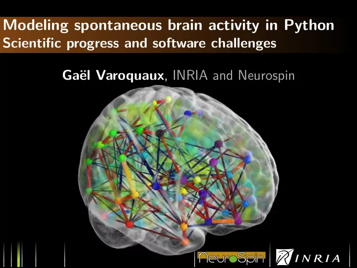
Modeling spontaneous brain activity in Python Scientific progress and software challenges Ga¨ el Varoquaux , INRIA and Neurospin
Spontaneous brain activity
Why study spontaneous brain activity? Explains 90% of the signal in task-driven experiments Window on intrinsic brain architecture Unique biomarker to study brain pathologies on impaired patients
Scientific challenge To develop in collaboration with neuroscientists new statistical tools to learn probabilistic models of spontaneous brain activity
Outline 1 Spatial patterns of brain activity 2 Beyond activation maps 3 Inter-subject comparisons 4 From models to software tools?
1 Spatial patterns of brain activity
1 Conventional brain mapping Study of stimuli response Mass-univariate statistics: for each voxel X = β β β Y + E Group inference: subject-variability model on β β β
1 Conventional brain mapping – software Nipy : NeuroImaging in Python Berkeley, Stanford, Neurospin . . . Vision: Open code shared between labs Progress: Statistical models implemented API difficult to use Good Input/Output code Preprocessing not implemented Roadblocks: Different teams ⇒ different visions Scientists can’t justify time on “solved problems”
1 Spatial correlation maps of spontaneous activity Biswal 1995: strong correlation between activity in left and right motor cortex at rest Later: seed-based correlation mapping The human brain is intrinsically organized into dynamic, anticorrelated functional networks (Fox 2005) How many? How to choose seeds?
1 Independent component analysis B : observed images = M : mixing matrix sources voxels sources voxels S : sources = B M · S Minimize mutual information between patterns S .
1 Independent component analysis B : observed images = M : mixing matrix sources voxels sources voxels S : sources = B M · S Minimize mutual information between patterns S .
1 Independent component analysis B : observed images = M : mixing matrix sources voxels sources voxels S : sources = B M · S Minimize mutual information between patterns S . No noise model ⇒ Lack of reproducibility + Fits noise
1 Model subject-to-subject variability A 1 A 2 � = Multivariate random effects model: Y s = loadings × P s + intra-subject noise PCA { P s } = loadings × B + inter-subject variability CCA B = M × A ICA ⇒ Group-level networks
1 Model subject-to-subject variability Reproducibility across random groups no CCA CCA + ICA Subspace .36 (.02) .71 (.01) One-to-one .36 (.02) .72 (.05) Varoquaux , NeuroImage 2010
1 Efficient Python implementation (CanICA) Problem to solve : ( 1 ) Y s = loadings × P s + . . . PCA: SVD ( 2 ) { P s } = loadings × B + . . . CCA: SVD ( 3 ) B = M × A ICA: iterations + Recomputed many times across random groups Step 2 and 3: Small data size ⇒ not bottleneck Step 1: Independent problems per subject ⇒ Parallel runs and caching of the results Joblib: Python functions as pipeline jobs Goals: remove dataflow and persistence problems from algorithmic code
Spatial patterns of brain activity New algorithms for spatial decomposition of spontaneous activity with explicit model of group-variability Separation of concerns in code: algorithms � = dataflow
2 Beyond activation maps
2 Segmenting sparse regions sources voxels sources voxels = M · S B
2 Segmenting sparse regions sources voxels sources voxels = M · S B sources voxels sources voxels voxels ( ( = B M · S Q + Interesting sources S sparse Q : Gaussian noise ⇒ Null hypothesis: centered normal distribution. Varoquaux , ISBI 2010
2 A full-brain parcellation Visual system map 0, reproducibility: 0.54 0 9 -74 V1 map 1, reproducibility: 0.52 -91 3 -3 V1-V2 map 3, reproducibility: 0.47 -80 40 4 extrastriate map 25, reproducibility: 0.34 -78 -30 24 superior parietal
2 A full-brain parcellation Motor system map 4, reproducibility: 0.47 part of -25 62 -1 motor map 21, reproducibility: 0.36 part of 54 -21 -42 motor map 32, reproducibility: 0.30 part of -8 -54 29 motor
2 A full-brain parcellation
2 Between-regions connectivity Correlation matrix Σ
Data Visualization Change of representation Understanding complex data requires inter- active visualization with high level concepts Mayavi: Python 3D visualization
3 Inter-subject comparisons
Ischemic stroke : Temporary interruption of blood flow Affects 1 person out of 100 every year for people > 55 years Causes focal lesions of varying consequences motor deficiencies language impairments coma . . . How does brain reorganize after stroke? Prognostic based on intrinsic brain activity?
3 Probabilistic covariance modeling Probabilistic model of data Covariance = 2 nd moment of observed data ⇒ Specifies a probability distribution Test the likelihood of data in a covariance model
3 Probabilistic covariance modeling Probabilistic model of data Covariance = 2 nd moment of observed data ⇒ Specifies a probability distribution Test the likelihood of data in a covariance model Covariances variations in healthy population Which one of the above has a large cortical lesion?
3 Probabilistic covariance modeling Probabilistic model of data Covariance = 2 nd moment of observed data ⇒ Specifies a probability distribution Test the likelihood of data in a covariance model Covariances variations in healthy population Which one of the above has a large cortical lesion?
3 Modeling variability of covariance Controls Patient Varoquaux , MICCAI 2010
3 Modeling variability of covariance Controls Patient Varoquaux , MICCAI 2010
3 Modeling variability of covariance Controls Patient Controls Patient Varoquaux , MICCAI 2010
3 Modeling variability of covariance Controls Patient dΣ Controls Patient P ( dΣ ) : probability density in tangent space Varoquaux , MICCAI 2010
3 Modeling variability of covariance Log-likelihood Controls Patient Tangent dΣ space Controls Patient controls patients P ( dΣ ) : probability density in tangent space Varoquaux , MICCAI 2010
3 Finding the cause of the difference Between which regions is connectivity is modified? Ill-posed problem Non-local effects ⇒ Many differences causes give the same observations Our suggestion Pair-wise partial correlations In tangent space: almost independent Draw random groups of healthy controls to tabulate their variability
3 Finding the cause of the difference
Research code in clinical settings Applications give rise to non-trivial mathematical problems Need to interact with neurologists Round-trips are costly: neurologists should use our code, modify our code
4 From models to software tools?
4 The hidden costs of releasing software Gap from paper to software: Remove duplication Write documentation Make usable APIs Write tests Fix corner cases Cost of code Complexity scales as the square of project size Woodfield 1979, an experiment on unit increase in problem complexity Cost of users Backward compatibility Support for multiple installations and versions Bug reports, feature request, mailing list support Maintenance cost ∼ ( # lines ) 2 √ # users
4 Addressing the scientific software challenge Better code High-level coding and abstractions numpy arrays: abstract out memory and pointers traits Model+View: hide dialogs and events joblib: factor out persistence Common libraries scipy, Mayavi, . . . Project management decisions 80/20 rule Not every research code should be released Focus on documentation and installation
4 Software as building blocks for new science Segregated, functionally-specialized, packages Answer a specific problem Limit dependencies Reusable projects Useful for a different purpose than the original one Libraries (no control of point of entry) Standard data structures Most often simple BSD licensed
4 Mayavi: making 3D visualization reusable Pipelines: from data sources to visualization objects ⇒ ⇒ ⇒ Simple API: mlab . contour3d ( x , y , z , data ) Building pipelines by function calls: mlab.pipeline.iso surface(mlab.pipeline.contour(src)) GUI + automatic script generation
4 Mayavi: making 3D visualization reusable 260 lines of code!
4 Mayavi: making 3D visualization reusable 260 lines of code! All dialogs are components: we expose our internals Visualizations included Traits view Easy update of data
4 joblib: not writing pipelines Dataflow pipeline: succession of processing steps executed on demand joblib : Lazy-revaluation Persitence Parallel processing Logging All with functions (seemingly)
4 joblib: not writing pipelines >>> from j o b l i b import Memory >>> mem = Memory ( c a c h e d i r =’/tmp/joblib ’) >>> import numpy as np >>> a = np . vander ( np . arange (3)) >>> s q u a r e = mem . cache ( np . s q u a r e ) >>> b = s q u a r e ( a ) [ Memory ] C a l l i n g s q u a r e ... s q u a r e ( a r r a y ([[0, 0, 1], [1, 1, 1], [4, 2, 1]])) s q u a r e - 0.0 s , 0.0 min >>> c = s q u a r e ( a ) >>> # The above call did not trigger an evaluation
Recommend
More recommend
Explore More Topics
Stay informed with curated content and fresh updates.

