Modeling Process Quality Statistical methodology plays an important - PowerPoint PPT Presentation
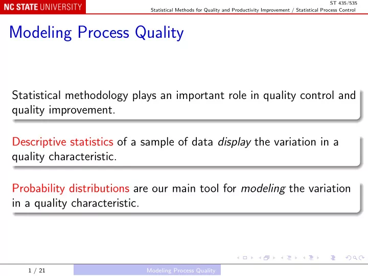
ST 435/535 Statistical Methods for Quality and Productivity Improvement / Statistical Process Control Modeling Process Quality Statistical methodology plays an important role in quality control and quality improvement. Descriptive statistics of
ST 435/535 Statistical Methods for Quality and Productivity Improvement / Statistical Process Control Modeling Process Quality Statistical methodology plays an important role in quality control and quality improvement. Descriptive statistics of a sample of data display the variation in a quality characteristic. Probability distributions are our main tool for modeling the variation in a quality characteristic. 1 / 21 Modeling Process Quality
ST 435/535 Statistical Methods for Quality and Productivity Improvement / Statistical Process Control Describing Variation Characteristics of the quality of goods and services always show variability. Examples: Net content of a can of a soft drink, when measured precisely; Time to complete an on-line banking transaction. We shall use both graphical and numerical tools to describe this variability. 2 / 21 Modeling Process Quality Describing Variation
ST 435/535 Statistical Methods for Quality and Productivity Improvement / Statistical Process Control Stem-and-Leaf Plot The stem-and-leaf display is a useful pencil-and-paper technique. Shows the distribution of data, like a histogram. Makes it easy to find the median, quartiles, and other quantiles (percentiles). Example 3.1 Table 3.1, Days to pay a health insurance claim In R: Table03p01 <- read.csv("Data/Table-03-01.csv"); stem(Table03p01$Days) 3 / 21 Modeling Process Quality Describing Variation
ST 435/535 Statistical Methods for Quality and Productivity Improvement / Statistical Process Control Time Series Plot The stem-and-leaf plot shows many aspects of the data, but not the time order . The time series plot is the same as a control chart. It can show: Shift in the mean; Trend; Change in variability. In R: plot(Days ~ Claim, data = Table03p01) # or simply plot(Table03p01$Days) 4 / 21 Modeling Process Quality Describing Variation
ST 435/535 Statistical Methods for Quality and Productivity Improvement / Statistical Process Control Histogram The number of leaves on each stem in a stem-and-leaf plot shows the distribution of the data. The histogram shows similar counts, with fewer restrictions on the bins. In R: hist(Table03p01$Days) hist(Table03p01$Days, right = FALSE) # same counts as in stem 5 / 21 Modeling Process Quality Describing Variation
ST 435/535 Statistical Methods for Quality and Productivity Improvement / Statistical Process Control Example 3.2 Table 3.2, thickness of vapor deposition layers on silicon In R: Table03p02 <- read.csv("Data/Table-03-02.csv"); hist(Table03p02$Thickness) # To look like Figure 3.3: hist(Table03p02$Thickness, right = FALSE, col = "brown", border = "white") 6 / 21 Modeling Process Quality Describing Variation
ST 435/535 Statistical Methods for Quality and Productivity Improvement / Statistical Process Control Numerical Summary of Data Graphical summaries like the stem-and-leaf plot and the histogram give a visual impression of the distribution of a set of data. Two key properties are: Central tendency; Dispersion. We also need numerical summaries of these properties. 7 / 21 Modeling Process Quality Describing Variation
ST 435/535 Statistical Methods for Quality and Productivity Improvement / Statistical Process Control For a set of observations x 1 , x 2 , . . . , x n , numerical summaries of central tendency include: The sample average � n x = x 1 + x 2 + · · · + x n i =1 x i ¯ = ; n n The sample median; Other trimmed means. In R: mean(Table03p01$Days) # 33.25 median(Table03p02$Thickness) # 450 mean(Table03p02$Thickness, trim = 0.25) # 449.94 8 / 21 Modeling Process Quality Describing Variation
ST 435/535 Statistical Methods for Quality and Productivity Improvement / Statistical Process Control The most common numerical summary of dispersion is the sample √ standard deviation s = s 2 , where n � x ) 2 ( x i − ¯ s 2 = i − 1 n − 1 is the sample variance . In R: sd(Table03p01$Days) # 9.374679 sd(Table03p02$Thickness) # 13.42732 9 / 21 Modeling Process Quality Describing Variation
ST 435/535 Statistical Methods for Quality and Productivity Improvement / Statistical Process Control Box Plot The box plot is a graphical display that shows 5 useful numerical summaries: The median; The two quartiles; The two extremes. It often also shows possible outliers. In R: # no outliers, whiskers extend to extremes: boxplot(Table03p01$Days) # possible outliers, whiskers extend only to non-outliers: boxplot(Table03p02$Thickness) 10 / 21 Modeling Process Quality Describing Variation
ST 435/535 Statistical Methods for Quality and Productivity Improvement / Statistical Process Control Comparison Box Plots Box plots are also useful for comparing multiple sets of data. In R: batteries <- read.csv("Data/batteries.csv"); boxplot(Life ~ Temperature, data = batteries) When a control chart is based on samples of characteristics, a comparison box plot is a good way to look for shifts in center or dispersion, possible outliers, and so on. 11 / 21 Modeling Process Quality Describing Variation
ST 435/535 Statistical Methods for Quality and Productivity Improvement / Statistical Process Control Probability Distributions We shall be working with two kinds of distribution: Discrete distributions, characterized by a probability mass function (pmf), like the binomial distribution; the pmf is p ( x i ) = P ( X = x i ) for each possible value x i . Continuous distributions, characterized by a probability density function (pdf), like the normal distribution; the pdf f ( x ) is interpreted through integrals: � b P ( a ≤ X ≤ b ) = f ( x ) dx . a 12 / 21 Modeling Process Quality Describing Variation
ST 435/535 Statistical Methods for Quality and Productivity Improvement / Statistical Process Control Mean and Variance The mean µ and variance σ 2 of a probability distribution are defined similarly to those of a sample : � ∞ i =1 x i p ( x i ) discrete X µ = � ∞ −∞ xf ( x ) dx continuous X i =1 ( x i − µ ) 2 p ( x i ) � ∞ discrete X σ 2 = � ∞ −∞ ( x − µ ) 2 f ( x ) dx continuous X 13 / 21 Modeling Process Quality Describing Variation
ST 435/535 Statistical Methods for Quality and Productivity Improvement / Statistical Process Control Examples # binomial pmf: plot(0:10, dbinom(0:10, size = 10, prob = 0.4), type = "h"); points(0:10, dbinom(0:10, size = 10, prob = 0.4)) # normal pdf: curve(dnorm(x), from = -3, to = 3) 14 / 21 Modeling Process Quality Describing Variation
ST 435/535 Statistical Methods for Quality and Productivity Improvement / Statistical Process Control Some Discrete Distributions Hypergeometric Distribution Sampling without replacement from a finite population. Population size N , of which D have some characteristic of interest. Sample size n . The random variable X is the number in the sample that are found to have that characteristic. Then the probability mass function is � D �� N − D � x n − x p ( x ) == , max(0 , n + D − N ) ≤ x ≤ min( n , D ) � N � n 15 / 21 Modeling Process Quality Important Discrete Distributions
ST 435/535 Statistical Methods for Quality and Productivity Improvement / Statistical Process Control The mean and variance are E( X ) = nD N and Var( X ) = nD � 1 − D � � N − n � N − 1 N N Application Acceptance sampling: N is lot size, D is number defective in the lot. 16 / 21 Modeling Process Quality Important Discrete Distributions
ST 435/535 Statistical Methods for Quality and Productivity Improvement / Statistical Process Control Binomial Distribution Sampling with replacement from a finite population, or sampling from an infinite population. A sequence of n independent trials, each of which results in “success” or “failure”. The probability of success in each trial is p . The random variable X is the number of successes found in the n trials. Then the probability mass function is � n � p x (1 − p ) n − x , 0 ≤ x ≤ n p ( x ) = P ( X = x ) = x 17 / 21 Modeling Process Quality Important Discrete Distributions
ST 435/535 Statistical Methods for Quality and Productivity Improvement / Statistical Process Control The mean and variance are E( X ) = np and Var( X ) = np (1 − p ) Sample fraction p = X The quantity ˆ n is the fraction of trials that result in success. p is the sample analog of the population probability p , and is the ˆ natural estimator of it. 18 / 21 Modeling Process Quality Important Discrete Distributions
ST 435/535 Statistical Methods for Quality and Productivity Improvement / Statistical Process Control Poisson Distribution Simplest model for random counts with no upper limit. For example, the number of blemishes in a new car’s paint. The probability mass function is p ( x ) = P ( X = x ) = e − λ λ x , x ≥ 0 x ! where λ is a positive parameter. The mean and variance are E( X ) = Var( X ) = λ 19 / 21 Modeling Process Quality Important Discrete Distributions
ST 435/535 Statistical Methods for Quality and Productivity Improvement / Statistical Process Control Negative Binomial and Geometric Distribution Recall the sequence of independent trials, each with success probability p . For some r > 0, the random variable X is the number of the trial when the r th success is seen. Then the probability mass function is � x − 1 � p r (1 − p ) x − r , x ≥ r p ( x ) = P ( X = x ) = r − 1 20 / 21 Modeling Process Quality Important Discrete Distributions
Recommend
More recommend
Explore More Topics
Stay informed with curated content and fresh updates.
