Modeling filter configuration Tyler Moore Computer Science & - PDF document

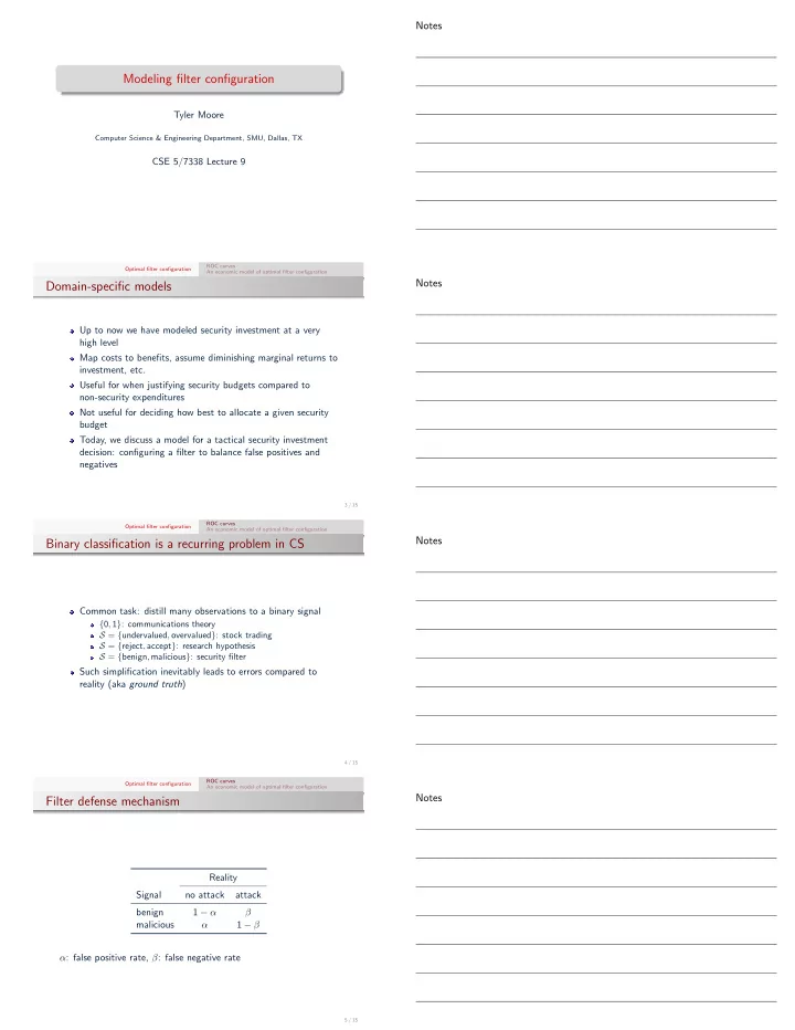
Notes Modeling filter configuration Tyler Moore Computer Science & Engineering Department, SMU, Dallas, TX CSE 5/7338 Lecture 9 ROC curves Optimal filter configuration An economic model of optimal filter configuration Notes Domain-specific models Up to now we have modeled security investment at a very high level Map costs to benefits, assume diminishing marginal returns to investment, etc. Useful for when justifying security budgets compared to non-security expenditures Not useful for deciding how best to allocate a given security budget Today, we discuss a model for a tactical security investment decision: configuring a filter to balance false positives and negatives 3 / 15 ROC curves Optimal filter configuration An economic model of optimal filter configuration Notes Binary classification is a recurring problem in CS Common task: distill many observations to a binary signal { 0 , 1 } : communications theory S = { undervalued , overvalued } : stock trading S = { reject , accept } : research hypothesis S = { benign , malicious } : security filter Such simplification inevitably leads to errors compared to reality (aka ground truth ) 4 / 15 ROC curves Optimal filter configuration An economic model of optimal filter configuration Notes Filter defense mechanism Reality Signal no attack attack benign 1 − α β malicious 1 − β α α : false positive rate, β : false negative rate 5 / 15

ROC curves Optimal filter configuration An economic model of optimal filter configuration Notes Receiver operating characteristic 1 Detection rate 1 − β 45 ◦ 0 1 False positive rate α 6 / 15 ROC curves Optimal filter configuration An economic model of optimal filter configuration Notes Receiver operating characteristic 1 Detection rate 1 − β α = β 45 ◦ 0 1 EER dashed EER solid False positive rate α 6 / 15 ROC curves Optimal filter configuration An economic model of optimal filter configuration Notes Model for optimal filter configuration Binary classifiers are imperfect Finding the optimal trade-off, say for an IDS or spam filter, is hard Can be framed as an economic trade-off between opportunity cost of false positives and losses incurred by false negatives 7 / 15 ROC curves Optimal filter configuration An economic model of optimal filter configuration Notes Model for optimal filter configuration We can see from ROCs that β can be expressed as a function of α . β : [0 , 1] → [0 , 1] defines the false negative rate as a function of the false positive rate α β (0) = 1 , β (1) = 0 We assume β ′ ( x ) < 0 and β ′′ ( x ) ≥ 0 8 / 15

ROC curves Optimal filter configuration An economic model of optimal filter configuration Notes Model for optimal filter configuration Suppose we rely on a filter to scan incoming email attachments for malware a : cost of false positive (blocking a benign email) b : cost of false negative (delivering malicious email) p : probability of email containing malware Cost C ( α ) = p · β ( α ) · b + (1 − p ) · α · a Suppose p = 0 . 1 , a = $250 , b = $500 , α = 0 . 1 , β = . 2 C ( α ) = 0 . 1 · 0 . 2 · 500 + 0 . 9 · 0 . 1 · 250 = $32 . 50 9 / 15 ROC curves Optimal filter configuration An economic model of optimal filter configuration Notes Optimal filter configuration: exercise 1 Suppose we rely on a filter to scan incoming email attachments for malware. Suppose the cost of dealing with a false negative event is $400, and the cost of dealing with a false positive is $200. 20% of incoming email has malware. You can choose between two configurations Config. A: 10% false positive rate and 30% false negative rate Config. B: 25% false positive rate and 15% false negative rate Your task: compute the expected costs for both configurations, and state which configuration you prefer. 10 / 15 ROC curves Optimal filter configuration An economic model of optimal filter configuration Notes Model for optimal filter configuration α ∗ = arg min α p · β ( α ) · b + (1 − p ) · α · a which has first-order condition (FOC) p · β ( α ∗ ) · b + (1 − p ) · α ∗ · a � � 0 = δ α after rearranging, we obtain: β ′ ( α ∗ ) = − 1 − p · a p b 11 / 15 ROC curves Optimal filter configuration An economic model of optimal filter configuration Notes Optimal filter configuration (continuous ROC curves) 1 (1 − p ) a p · b Detection rate 1 − β α ∗ B Indifference curves α ∗ A 0 False positive rate α 1 12 / 15

ROC curves Optimal filter configuration An economic model of optimal filter configuration Notes Optimal filter configuration (continuous ROC curves) A 1 B Detection rate 1 − β EER A = EER B α = β AUC A = AUC B 45 ◦ 0 False positive rate α 1 12 / 15 ROC curves Optimal filter configuration An economic model of optimal filter configuration Notes Optimal filter configuration (continuous ROC curves) A 1 B (1 − p ) a p · b Detection rate 1 − β α ∗ B α ∗ A 45 ◦ 0 False positive rate α 1 12 / 15 ROC curves Optimal filter configuration An economic model of optimal filter configuration Notes Optimal filter configuration (discrete ROC curves) 1 E F (1 − p ) a p · b Detection rate 1 − β α ∗ D 45 ◦ C 0 False positive rate α 1 13 / 15 ROC curves Optimal filter configuration An economic model of optimal filter configuration Notes Optimal filter configuration example (discrete ROC curves) slope 1/3 1 E F 0.1 0.3 0.9 Detection rate 1 − β (1 − p ) a p · b 1 0.5 e p o l s α ∗ D 0.5 0.4 2 α ∗ = 0 . 2 if 1 ≤ (1 − p ) a e ≤ 2 0.4 p p · b o l s C 0.2 0.2 0.7 0 1 False positive rate α 14 / 15

ROC curves Optimal filter configuration An economic model of optimal filter configuration Notes Optimal filter configuration: exercise 2 Suppose we rely on a filter to scan incoming email attachments for malware. Suppose the cost of dealing with a false negative event is $400, and the cost of dealing with a false positive is $200. 20% of incoming email has malware. You can choose between two configurations Config. A: 10% false positive rate and 30% false negative rate Config. B: 25% false positive rate and 15% false negative rate Your task Draw the ROC curve for configurations A and B (plus (0% FP, 1 100% FN) and (100% FP, 0% FN)) Calculate the slope of the indifference curve for the optimal 2 configuration Select the optimal point for the ROC curve 3 15 / 15 Notes Notes Notes