Modeling business and financial cycle in a multivariate structural - PowerPoint PPT Presentation

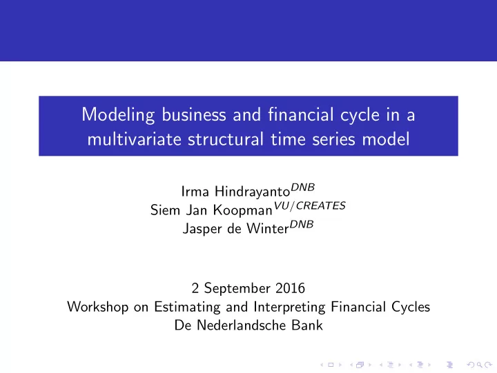
Modeling business and financial cycle in a multivariate structural time series model Irma Hindrayanto DNB Siem Jan Koopman VU / CREATES Jasper de Winter DNB 2 September 2016 Workshop on Estimating and Interpreting Financial Cycles De Nederlandsche Bank

Presentation Outline 1 Introduction 2 Modeling approach 3 Empirical results 4 Conclusions

Introduction Financial cycles have become a popular topic since the great crisis of 2008. Renewed interest in the ‘credit cycle’ and research into cycles in other financial variables. Several methods have been proposed, such as band-pass filters, turning point analysis, continuous wavelet analysis, and also model-based time series analysis. We focus on applying multivariate unobserved components model in order to extract these cycles. Key feature: we extract both short- and medium-term cycles in one framework (as in Koopman & Lucas (2005) and Chen et al (2012)).

Previous related studies Galati et al (2016) 1 applied unobeserved components model analysis to credit-to-GDP ratio, real credit and real house prices, 2 found not one common financial cycle but several similar financial cycles (meaning having the same frequency and degree of persistence, but different variances in the stochastic part of the model), 3 which tend to be longer and have larger amplitudes than what is commonly found for business cycles.

Previous related studies R¨ unstler & Vlekke (2016) 1 applied multivariate filter to capture the medium-term cycles of real GDP, real credit and real house prices, 2 added an extra lag on the cycle specification to get better diagnostics, 3 found long and large cycles in credit and house prices, but they differ siginicantly across countries, 4 point out that financial cycles are closely correlated with the medium-term cycle of GDP.

Our Research Questions 1 How to relate the business cycle to the financial cycles’ developments? Comin & Gertler (2006): many industrialized countries have experienced significant medium-term oscillations. However, the conventional business cycle filters tend to sweep these movement into the trend. Crowley (2010): great moderation is only evident in the shorter cycles and does not affect the amplitude of the longer cycles. 2 Is it possible to simultaneously extract these two cycles from several macroeconomics and financial variables in a not too complicated model? 3 Is it possible to interpret the literatures using these two types of cycles?

Multivariate Unobserved Component Model Framework Model specification as in Koopman and Lucas (2005): i . i . d . ∼ N (0 , Σ ε ) , y t = µ t + A γ t + B ψ t + ε t , ε t (1) y t : time series in a panel with length of N . µ t : long-term trend. γ t : short-term cycle. ψ t : medium-term cycle. ε t : noise. The loading matrices A and B reveal whether there is some co-cyclicality between the series in the panel.

Modeling the Trend Key part of the analysis → getting the appropriate smoothness of the trend component (how much fluctuation in y t is assigned to the trend as opposed to other components). We use the integrated random walk process: µ t +1 = µ t + β t , (2) i . i . d . β t +1 = β t + ζ t , ζ t ∼ N (0 , Σ ζ ) , with restriction on the signal-to-noise ratio: σ 2 ζ /σ 2 ε = 0 . 000625.

Modeling the Cycles AR(2) which allows the polynomial autoregressive coefficients to have complex roots: � ψ t +1 � � ψ t � ω t � � cos λ ψ I N sin λ ψ I N � � = φ ψ + , ψ ∗ − sin λ ψ I N cos λ ψ I N ψ ∗ ω ∗ t +1 t t � ω t � i . i . d . ∼ N (0 , I 2 ⊗ D ω ) (3) ω ∗ t ψ t = cycle, ψ ∗ t = ‘first derivative of cycle’, λ ψ = cycle frequency, φ ψ = persistence parameter, ω t = disturbance term. The length of ψ t is given by p = 2 π/λ ψ . For identification of the cycle disturbance variances, A and B in Eq.(1) are restricted to be lower triangular matrices with unity as diagonal elements.

State Space Form The multivariate components model (1)-(4) can be cast into the state space form α t = T α t − 1 + ν t , y t = Z α t + ε t , where the state vector α t contains the unobservables t , γ ∗ ′ t , ψ ∗ ′ ( µ t , β t , γ ′ t , ψ ′ t ) ′ . Z and T are constructed according to the specifications implied by the model. The state disturbances vector ν t contains ζ t , κ t , κ ∗ t , ω t and ω ∗ t .

Empirical analysis set-up We apply the multivariate UC model to extract trends and cycles from the following variables: real gross domestic product (GDP), real house prices (HP), real bank credit to private sector (CRED), and industrial production index (IP). Data source: BIS, OECD, IMF. The countries in our sample are US, UK, JA, CA, DE, FR, IT (the so-called G7 countries) and NL over the period of 1970Q1 to 2015Q4, with monthly data for IP series. We incorporate both quarterly and monthly series into one multivariate framework. Warning: It is difficult to separate the medium-term cyclical movements from the trend.

Summary of short-term cycle parameter estimates Table: Commonality between GDP and other short -term cycles US UK JA CA DE FR IT NL p γ 4.08 6.78 3.27 6.3 3.73 5.71 3.13 8.11 φ γ 0.97 0.97 0.97 0.98 0.97 0.98 0.97 0.99 HP -0.21 1.00 0.48 1.52 0.04 0.47 -0.17 0.51 CRED 0.32 0.17 -0.06 0.83 -0.12 0.31 0.27 0.76 IP 1.82 1.90 3.73 2.81 2.94 2.97 2.43 1.62

Results on the short-term cycle 1 Averaged over all countries in the sample, the average duration of the short-term cycle is 5.2 years. NL has the longest short cycle: 8.2 years. IT has the shortest duration: 3.1 years. 2 There is a strong evidence for short-term co-cyclicality between GDP and IP in all the countries that we considered. 3 We found weak evidence for short-term co-cyclicality between GDP and house prices. Only UK and CA have a significant loading. 4 We found very little evidence for commonality between the short-term credit and GDP cycles. Only NL has a significant loading.

Summary of medium-term cycle parameter estimates Table: Commonality between GDP and other medium -term cycles US UK JA CA DE FR IT NL ∗ p ψ 12.92 15.08 8.61 25.8 8.48 17.62 14.13 20.60 φ ψ 0.99 0.99 0.99 0.99 0.99 0.99 0.99 0.99 HP 2.30 8.18 1.47 -0.41 0.66 2.80 0.73 15.40 CRED 2.40 4.05 1.85 0.09 0.75 2.55 0.64 4.33 IP 2.07 0.26 2.76 1.03 2.23 2.22 2.37 2.79

Results on the medium-term cycle 1 The average duration of the medium-term cycle varies from 8.5 years in DE to 20.6 years in NL. 2 For most countries, the medium-term cycle is dominant in explaining the cyclical variability for the financial variables (credit and house prices). 3 There is evidence of strong medium-term co-cyclicality between house prices and GDP or credit and GDP for most countries. Exceptions are CA, DE and IT. 4 In NL the medium-term co-cylicality between credit and GDP goes indirectly via house prices. Thus medium-term credit cycle shares commonality with the house prices cycle, which in turn shares commonality with GDP cycle.

Conclusions for G7 countries and NL 1 Based on the multivariate unobserved component model analysis, we estimated short- and medium-term cycles in GDP, house prices, credit and industrial production index. 2 Industrial production index seems to be the driver of the short-term cycles. 3 The house prices and credit tend to dominate the medium-term cycles. 4 Results vary across countries, but there are also many similarities. 5 We support the statement in Crowley (2010) for the US: great moderation seems to be only evident in the shorter cycles and does not affect the amplitude of the longer cycles.

Multivariate UC model analysis for US 9.5 5.00 5.0 House Price House Price Credit Credit GDP GDP Industrial Production Industrial Production µ t µ t µ t µ t µ t µ t µ t µ t 9.5 4.75 9.0 4.5 4.50 9.0 8.5 4.0 4.25 8.0 8.5 1970 1985 2000 2015 1970 1985 2000 2015 1970 1985 2000 2015 1970 1985 2000 2015 0.05 γ t γ t γ t γ t γ t γ t 0.02 γ t γ t 0.01 0.02 0.00 0.00 0.00 0.00 -0.05 -0.01 -0.02 1970 1985 2000 2015 1970 1985 2000 2015 1970 1985 2000 2015 1970 1985 2000 2015 0.2 ψ t ψ t ψ t ψ t ψ t ψ t ψ t ψ t 0.05 0.025 0.1 0.1 0.000 0.0 0.0 0.00 -0.1 -0.025 -0.1 -0.05 1970 1985 2000 2015 1970 1985 2000 2015 1970 1985 2000 2015 1970 1985 2000 2015

Multivariate UC model analysis for UK 5.0 4.75 GDP GDP House Price House Price Credit Credit Industrial Production Industrial Production µ t µ t µ t µ t µ t µ t µ t µ t 7 4.5 14.0 4.50 4.0 6 3.5 13.5 4.25 1979 1999 1980 2000 1980 2000 1980 2000 0.1 0.05 0.025 γ t γ t γ t γ t γ t γ t γ t γ t 0.1 0.000 0.0 0.00 0.0 -0.025 1980 2000 1980 2000 1980 2000 1980 2000 ψ t ψ t 0.2 ψ t ψ t ψ t ψ t ψ t ψ t 0.025 0.2 0.005 0.000 0.000 0.0 0.0 -0.005 -0.025 -0.2 1980 2000 1980 2000 1980 2000 1980 2000