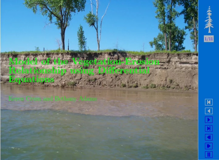

1/11 Model of the Vegetation-Erosion Relationship using Differential Equations Keren Crum and Bethany Adams � � � � � � �
Vegetation-Erosion Dynamics • Vegetation-Erosion Dynamics study the relationship between the Vegetation Coverage Density (VCD) of an area to its rate of Erosion 2/11 • There is an inverse relationship between VCD and erosion in that the higher the VCD the less erosion, while the higher the erosion the harder for vegetation to take hold. • Vegetation-Erosion Dynamics also integrate the effects of natural forces and human interactions on the change in VCD and Erosion of an area • Erosion is a serious problem that affects the farmlands and natural � habitats. � • Models predict the long-term nature of watersheds � • Models show the negative and positive influences humans have on � VE dynamics and provide analysis to devise a plan of action to � improve the ecosystem. � �
Vegetation-Erosion Dynamics Model The basic equation for Vegetation-Erosion dynamics is given by 3/11 dV dt = aV − cE (1) dE dt = dE − fV where V and E represent the percentage of vegetation-coverage and the rate of erosion in ton/km 2 respectively. The coefficients a , c , d , and f are the natural rates of VCD, erosion, erosion effects that further erosion, and vegetation coverage that re- � duces erosion, which are specific to the area. � � � � � �
Vegetation-Erosion Dynamics Model Natural and human stresses on vegetation and erosion must also be evaluated to create a complete model giving us the linear differential 4/11 equation model with forcing terms of V τ and E τ dV dt = aV − cE + V τ (2) dE dt = dE − fV + E τ where E τ represents human affects on erosion V τ represents natural and human ecological stresses. � � � � � � �
Solving the Equation The solution to the linear differential equations (2) is given by the homogeneous solution plus the nonhomogeneous solution 5/11 V = c 1 e λ 1 t + c 2 e λ 2 t + V 1 ( t ) (3) a − λ 1 a − λ 2 e λ 1 t + c 2 e λ 2 t + E 1 ( t ) E = c 1 c c where c 1 and c 2 are constants determined from the initial conditions and λ 1 and λ 2 are eigenvalues in terms of the coefficients a,c,d, and f given by � λ 1 = ( a + d ) − ( a + d ) 2 − 4( ad − cf ) � 2 � (4) � λ 2 = ( a + d ) + ( a + d ) 2 − 4( ad − cf ) � . 2 � � � �
Qualitative Analysis Now that we have solved our equations we can use qualitative analy- sis to determine the current condition of the system and the likelihood 6/11 of the ecological system to recover or deteriorate. Using the equations (2) from our original system, we can find the nullclines of the system by setting dV/dt and dE/dt equal to zero and solving for E . E = a cV + 1 cV τ (5) E = f dV − 1 dE τ � � � � � � �
Vegetation-Erosion Chart Evaluating the vegetation density versus the erosion produces a Vegetation-Erosion Chart. 7/11 Unstressed Vegetation−Erosion Chart Stressed Vegetation−Erosion Chart 3 3 E=aV/c E=aV/c+V tau /c Erosion Level (1000 ton/km 2 year) Erosion Level (1000 ton/km 2 year) A E=fV/d 2.5 2.5 E=fV/d−E tau /d A 2 2 B 1.5 1.5 B 1 1 � C C .5 .5 � � 0 0 0 0.5 1 0 0.5 1 Vegetation Cover Density (%) Vegetation Cover Density (%) � � � �
Heishui River Basin The Heishui River Basin is a small tributary of the Yangtze river that was targeted as a study for erosion control due to its high erosion 8/11 rates of 7,243 ton/km 2 per year and low vegetation coverage of 7.6%. Beginning in 1978 the government reforested the river basin at a rate of 4% per year( V τ 0 ), while also installing erosion control dams that reduced erosion by 650 ton/km 2 per year( E τ 0 ). The ecological stresses in this case are constant where V τ ( t ) = V τ 0 and E τ ( t ) = E τ 0 , (6) Evaluating the solution from (3) gives the equations � � V ( t ) = c 1 e λ 1 t + c 2 e λ 2 t − dV τ 0 + cE τ 0 � ad − cf (7) � a − λ 1 a − λ 2 e λ 2 t + − fV τ 0 + aE τ 0 e λ 1 t + c 2 E ( t ) = c 1 � c c ad − cf � �
Heishui: Qualitative Analysis The Vegetation-Erosion Chart of the Heishui model demonstrates how improving vegetation and erosion conditions decrease the high 9/11 risk (A) and the medium risk (B) sections. Vegetation−Erosion Dynamics Chart Vegetation−Erosion Dynamics Chart without Erosion Control with Erosion Control 16 16 A Erosion Level (1000 tons/km 2 year) Erosion Level (1000 tons/km 2 year) dV/dt=0 dE/dt=0 A B 12 12 C B 8 8 � � 4 4 dV/dt=0 � C dE/dt=0 0 0 � 0 0.5 1 0 0.5 1 Vegetation Cover Density (%) Vegetation Cover Density (%) � � �
Heishui Graphs Using the initial conditions of V (1978) = . 076 E (1978) = 7 , 243 we can simulate the activity of the Vegetation Coverage and the Erosion 10/11 in the Heishui Basin. Vegetation Cover Density over Time Erosion over Time 1 20 Model w/ Erosion Control Model w/ Erosion Control Model w/o Erosion Control Model w/o Erosion Control Erosion (1000 tons/km 2 year 0.8 16 Actual VCD Actual Erosion Vegetation Cover (%) 0.6 12 0.4 8 � � 0.2 4 � 0 0 1980 1985 1990 1995 1980 1985 1990 1995 � Year Year � We simulated the model with and without erosion control along with � the measured to show the importance of erosion control. �
Conclusion • Vegetation-Erosion Dynamics is a relatively new area in science that has shown the important interconnectedness of vegetation to 11/11 erosion. • Human activities have a great impact on the environment and should take responsibility to sustain a vibrant ecosystem. • Vegetation-Erosion models can help determine the current condi- tions and help develop effective means to reduce erosion. • Vegetation-Erosion analysis will eventually be incorporated into civil engineering projects to help minimize impacts to the environ- � ment. � � � � � �
Recommend
More recommend