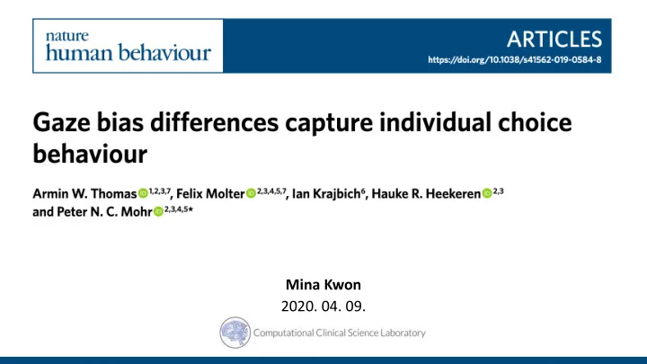
Mina Kwon 2020. 04. 09. vs vs Preference Gaze influence - PowerPoint PPT Presentation
Mina Kwon 2020. 04. 09. vs vs Preference Gaze influence Fixation Choice A HIGH B LOW Dataset Dataset Task description Dataset Task description Set size Binary choice Dataset Task description Set size Trinary choice Dataset
Mina Kwon 2020. 04. 09.
vs
vs Preference Gaze influence Fixation Choice A HIGH B LOW
Dataset
Dataset Task description
Dataset Task description Set size Binary choice
Dataset Task description Set size Trinary choice
Dataset Task description Choice domain Value-based choice
Dataset Task description Choice domain Perceptional choice
Behavioral data
Behavioral data Three behavioral metrics ● Mean RT (Mean response time) Value-based task (a, b, c) : item with higher likeness rating ● P(choosing best) (Mean probability of choosing the best item) Perceptional task (d) : item with smaller angular distance ● Gaze influence 1) Probability of choosing the item : based on item value Observed data 2) Residual choice probability = observed data – probability of choosing the item (1: chosen, 0: otherwise) 3) Gaze influence on choice = 𝑞𝑝𝑡𝑗𝑢𝑗𝑤𝑓 𝑏𝑨𝑓 𝑏𝑒𝑤𝑏𝑜𝑢𝑏𝑓 ’s Residual choice probability – 𝑜𝑓𝑏𝑢𝑗𝑤𝑓 𝑏𝑨𝑓 𝑏𝑒𝑤𝑏𝑜𝑢𝑏𝑓 ’s Residual choice probability * 𝑞𝑝𝑡𝑗𝑢𝑗𝑤𝑓 𝑏𝑨𝑓 𝑔𝑗𝑜𝑏𝑚 𝑏𝑒𝑤𝑏𝑜𝑢𝑏𝑓 : fraction of time fixated on the item > average fixated time for the others * 𝑜𝑓𝑏𝑢𝑗𝑤𝑓 𝑏𝑨𝑓 𝑔𝑗𝑜𝑏𝑚 𝑏𝑒𝑤𝑏𝑜𝑢𝑏𝑓 : fraction of time fixated on the item < average fixated time for the others
Behavioral data Behavioral Results Individual difference in the behavioral metrics Positive Gaze influence score: 98% Gaze influence: -11% ~ 72% Associations between the behavioral metrics ↑ Gaze influence, ↓ p(choosing best) Fig. 2
Computational model
Computational model GLAM: Gaze-weighted Linear Accumulator Model ● Linear stochastic horse race model b For more information about previous DDM (Ian Krajbich et al., 2010; 2011; 2012; 2015)
Computational model GLAM: Gaze-weighted Linear Accumulator Model ● Linear stochastic horse race model b For more information about previous DDM (Ian Krajbich et al., 2010; 2011; 2012; 2015)
Computational model GLAM: Gaze-weighted Linear Accumulator Model Accumulated relative evidence 𝜉 = velocity parameter (speed of accumulation) 𝑢 = time point 𝜏 = standard deviation 𝑆 = Drift term Logistic transformation Drift term Relative evidence Stationary absolute evidence signal 𝑈𝑝𝑢𝑏𝑚 𝑔𝑗𝑦𝑏𝑢𝑗𝑝𝑜 𝑝𝑜 𝑗𝑢𝑓𝑛 𝑗 ! = relative gaze = 𝑈𝑝𝑢𝑏𝑚 𝑔𝑗𝑦𝑏𝑢𝑗𝑝𝑜 𝑠 ! = item value 𝛿 = 1 : No gaze bias 𝛿 = gaze bias parameter 𝛿 < 1 : Gaze bias
Computational model GLAM: Gaze-weighted Linear Accumulator Model Accumulated relative evidence 𝜉 = velocity parameter (speed of accumulation) 𝑢 = time point 𝜏 = standard deviation 𝑆 = Drift term Logistic transformation Drift term scaling parameter Relative evidence Stationary absolute evidence signal 𝑈𝑝𝑢𝑏𝑚 𝑔𝑗𝑦𝑏𝑢𝑗𝑝𝑜 𝑝𝑜 𝑗𝑢𝑓𝑛 𝑗 ! = relative gaze = 𝑈𝑝𝑢𝑏𝑚 𝑔𝑗𝑦𝑏𝑢𝑗𝑝𝑜 𝑠 ! = item value 𝛿 = 1 : No gaze bias 𝛿 = gaze bias parameter 𝛿 < 1 : Gaze bias
Computational model GLAM: Gaze-weighted Linear Accumulator Model Accumulated relative evidence Distribution of Gaze 𝜉 = velocity parameter (speed of accumulation) 𝑢 = time point 𝜏 = standard deviation 𝑆 = Drift term Logistic transformation Drift term Relative evidence Stationary absolute evidence signal 𝑈𝑝𝑢𝑏𝑚 𝑔𝑗𝑦𝑏𝑢𝑗𝑝𝑜 𝑝𝑜 𝑗𝑢𝑓𝑛 𝑗 ! = relative gaze = 𝑈𝑝𝑢𝑏𝑚 𝑔𝑗𝑦𝑏𝑢𝑗𝑝𝑜 𝑠 ! = item value 𝛿 = 1 : No gaze bias 𝛿 = gaze bias parameter 𝛿 < 1 : Gaze bias
Computational model GLAM: Gaze-weighted Linear Accumulator Model Accumulated relative evidence 𝜉 = velocity parameter (speed of accumulation) 𝑢 = time point 𝜏 = standard deviation 𝑆 = Drift term Logistic transformation Drift term Relative evidence Stationary absolute evidence signal 𝑈𝑝𝑢𝑏𝑚 𝑔𝑗𝑦𝑏𝑢𝑗𝑝𝑜 𝑝𝑜 𝑗𝑢𝑓𝑛 𝑗 ! = relative gaze = 𝑈𝑝𝑢𝑏𝑚 𝑔𝑗𝑦𝑏𝑢𝑗𝑝𝑜 𝑠 ! = item value 𝛿 = 1 : No gaze bias 𝛿 = gaze bias parameter 𝛿 < 1 : Gaze bias
Computational model GLAM: Gaze-weighted Linear Accumulator Model Accumulated relative evidence 𝜉 = velocity parameter (speed of accumulation) 𝑢 = time point 𝜏 = standard deviation 𝑆 = Drift term Logistic transformation Drift term Logistic transformation Relative evidence Stationary absolute evidence signal 𝑈𝑝𝑢𝑏𝑚 𝑔𝑗𝑦𝑏𝑢𝑗𝑝𝑜 𝑝𝑜 𝑗𝑢𝑓𝑛 𝑗 ! = relative gaze = 𝑈𝑝𝑢𝑏𝑚 𝑔𝑗𝑦𝑏𝑢𝑗𝑝𝑜 𝑠 ! = item value 𝛿 = 1 : No gaze bias 𝛿 = gaze bias parameter 𝛿 < 1 : Gaze bias
Computational model GLAM: Gaze-weighted Linear Accumulator Model Accumulated relative evidence 𝜉 = velocity parameter (speed of accumulation) 𝑢 = time point 𝜏 = standard deviation 𝑆 = Drift term Logistic transformation Drift term Relative evidence Stationary absolute evidence signal 𝑈𝑝𝑢𝑏𝑚 𝑔𝑗𝑦𝑏𝑢𝑗𝑝𝑜 𝑝𝑜 𝑗𝑢𝑓𝑛 𝑗 ! = relative gaze = 𝑈𝑝𝑢𝑏𝑚 𝑔𝑗𝑦𝑏𝑢𝑗𝑝𝑜 𝑠 ! = item value 𝛿 = 1 : No gaze bias 𝛿 = gaze bias parameter 𝛿 < 1 : Gaze bias
Computational model GLAM: Gaze-weighted Linear Accumulator Model 𝑄 % 𝑢 : Probability of 𝐹 % reaching 𝑐 at time 𝑢 , before any other accumulator has reached.
Computational model GLAM: Gaze-weighted Linear Accumulator Model 𝑄 % 𝑢 : Probability of 𝐹 % reaching 𝑐 at time 𝑢 , before any other accumulator has reached. Resulting choice likelihood
Computational results
Computational results Parameter recovery S. Fig. 7: Results of a parameter recovery study of the GLAM
Computational results Presence of individual difference in gaze bias Fig. 4 S. Fig. 1 Individual parameter estimates of 𝜹 Model comparison using WAIC (Widely Applicable Information Criterion) [-1.03 ~ 0.97] 1) Full GLAM model 2) No-Gaze-bias GLAM variant (gaze bias parameter 𝛿 = 1) è Non-trivial difference in Gaze bias! è Full GLAM model fitted 109/118 participants (98%) better than No bias model
Computational results Model simulation ● Predicted choices (3 behavioral metrics) & RT - Train set: Even-numbered trials - Test set: Odd-numbered trials Full GLAM No-Gaze-Bias Model Fig. 5 S. Fig. 5 & 6 Choice prediction RT prediction
Computational results Model simulation ● Behavioral metrics prediction Fig. 2 S. Fig. 4 Out-of-sample predicted data Observed data
Computational results Individual’s response behavior & parameter ● Associations between the model parameters & response behavior a. ↑ velocity parameter , ↓ mean RT b. ↑ Gaze influence ( ↓ 𝛿 ), ↑ Gaze influence score c. ↑ Gaze influence ( ↓ 𝛿 ), ↓ p(choosing best) Fig. 6
Discussion
Discussion Summary ● Test the model GLAM using 4 different datasets. 1) Compared model with & without gaze bias è Individual variability in gaze bias exists, since model with bias better explained individual’s choice behavior. 2) Model simulation of GLAM è GLAM accurately predicted observed behavioral data and their associations. 3) Associations between the model parameter & behavioral data è Stronger gaze influence in the model was associated with stronger gaze influence score & inconsistent choice with item value in individuals’ response.
Discussion Strength & Implication ● GLAM enables trial specific prediction and prediction in Multiple choice situation. ● GLAM doesn’t require a simulation of eye movement. ● Analyses span across two set sizes & two choice domains. ● Found individual difference in influence of gaze on choice behavior. è Are these differences trait, state, or both?
Reference
Reference Krajbich, I., Armel, C., & Rangel, A. (2010). Visual fixations and the computation and comparison of value in simple choice. Nature Neuroscience , 13 (10), 1292–1298. https://doi.org/10.1038/nn.2635 Krajbich, I., Lu, D., Camerer, C., & Rangel, A. (2012). The attentional drift-diffusion model extends to simple purchasing decisions. Frontiers in Psychology , 3 , 193. https://doi.org/10.3389/fpsyg.2012.00193 Krajbich, I., & Rangel, A. (2011). Multialternative drift-diffusion model predicts the relationship between visual fixations and choice in value- based decisions. Proceedings of the National Academy of Sciences of the United States of America , 108 (33), 13852–13857. https://doi.org/10.1073/pnas.1101328108 Krajbich, I., & Smith, S. M. (2015). Modeling Eye Movements and Response Times in Consumer Choice. Journal of Agricultural & Food Industrial Organization , 13 (1), 55–72. https://doi.org/10.1515/jafio-2015-0016
Thank you
Additional Slides
Recommend
More recommend
Explore More Topics
Stay informed with curated content and fresh updates.
