Methods for Partitioning Data to Improve Parallel Execution Time for - PowerPoint PPT Presentation

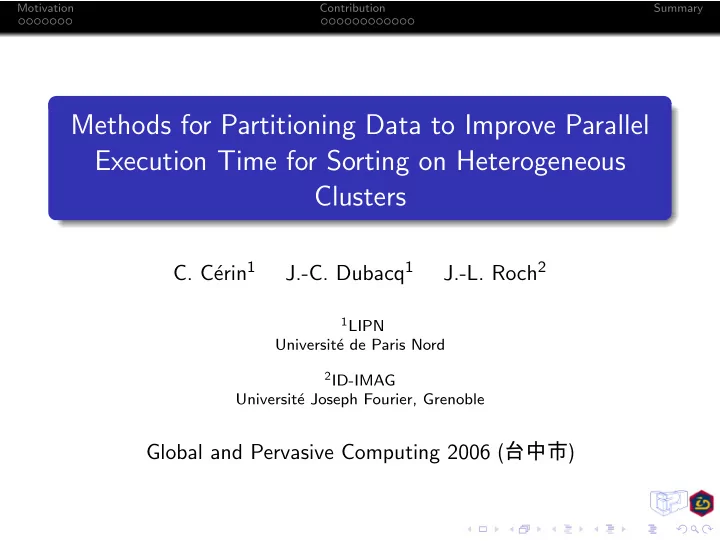
Motivation Contribution Summary Methods for Partitioning Data to Improve Parallel Execution Time for Sorting on Heterogeneous Clusters erin 1 J.-C. Dubacq 1 J.-L. Roch 2 C. C´ 1 LIPN Universit´ e de Paris Nord 2 ID-IMAG Universit´ e Joseph Fourier, Grenoble Global and Pervasive Computing 2006 ( 台 中 市 )

Motivation Contribution Summary Outline Motivation 1 The partitioning problem Splitting data Contribution 2 General exact analytic approach Dynamic evaluation of complexity function Non uniformly related processors Experiments

Motivation Contribution Summary Outline Motivation 1 The partitioning problem Splitting data Contribution 2 General exact analytic approach Dynamic evaluation of complexity function Non uniformly related processors Experiments

Motivation Contribution Summary Partitioning large data sets for sorting Large data sets require lot of computation time for sorting;

Motivation Contribution Summary Partitioning large data sets for sorting Large data sets require lot of computation time for sorting; Data chunks of equal size used to do the job on parallel machines.

Motivation Contribution Summary Partitioning large data sets for sorting Large data sets require lot of computation time for sorting; Data chunks of equal size used to do the job on parallel machines. Modelisation Infinite point-to-point bandwidth;

Motivation Contribution Summary Partitioning large data sets for sorting Large data sets require lot of computation time for sorting; Data chunks of equal size used to do the job on parallel machines. Modelisation Infinite point-to-point bandwidth; Heterogeneous speed: relative linear speed;

Motivation Contribution Summary Partitioning large data sets for sorting Large data sets require lot of computation time for sorting; Data chunks of equal size used to do the job on parallel machines. Modelisation Infinite point-to-point bandwidth; Heterogeneous speed: relative linear speed; No study of memory effect.

Motivation Contribution Summary Methodology 1 Data chunks are sent from node 0 to nodes 1 , . . . , p − 1;

Motivation Contribution Summary Methodology 1 Data chunks are sent from node 0 to nodes 1 , . . . , p − 1; 2 Each processor sorts locally its data chunk;

Motivation Contribution Summary Methodology 1 Data chunks are sent from node 0 to nodes 1 , . . . , p − 1; 2 Each processor sorts locally its data chunk; 3 Node 0 receives p − 1 pivots, sorts them and broadcasts them;

Motivation Contribution Summary Methodology 1 Data chunks are sent from node 0 to nodes 1 , . . . , p − 1; 2 Each processor sorts locally its data chunk; 3 Node 0 receives p − 1 pivots, sorts them and broadcasts them; 4 Each processor uses the pivots to split its data;

Motivation Contribution Summary Methodology 1 Data chunks are sent from node 0 to nodes 1 , . . . , p − 1; 2 Each processor sorts locally its data chunk; 3 Node 0 receives p − 1 pivots, sorts them and broadcasts them; 4 Each processor uses the pivots to split its data; 5 Each processor transmits all its (split) data to the others;

Motivation Contribution Summary Methodology 1 Data chunks are sent from node 0 to nodes 1 , . . . , p − 1; 2 Each processor sorts locally its data chunk; 3 Node 0 receives p − 1 pivots, sorts them and broadcasts them; 4 Each processor uses the pivots to split its data; 5 Each processor transmits all its (split) data to the others; 6 Each processor merges all data it received with its own.

Motivation Contribution Summary Methodology 1 Data chunks are sent from node 0 to nodes 1 , . . . , p − 1; 2 Each processor sorts locally its data chunk; 3 Node 0 receives p − 1 pivots, sorts them and broadcasts them; 4 Each processor uses the pivots to split its data; 5 Each processor transmits all its (split) data to the others; 6 Each processor merges all data it received with its own. Observation With fixed p, the computation-intensive part is step 2.

Motivation Contribution Summary Context: Grid’5000, heterogeneous clusters GRID’5000: French national research project on grids;

Motivation Contribution Summary Context: Grid’5000, heterogeneous clusters GRID’5000: French national research project on grids; Goal: 5000 nodes dedicated to experimental development;

Motivation Contribution Summary Context: Grid’5000, heterogeneous clusters GRID’5000: French national research project on grids; Goal: 5000 nodes dedicated to experimental development; Current state: 2300 nodes, 13+ separated clusters, 9 sites, dedicated 10 Gb/s black fibre connexion;

Motivation Contribution Summary Context: Grid’5000, heterogeneous clusters GRID’5000: French national research project on grids; Goal: 5000 nodes dedicated to experimental development; Current state: 2300 nodes, 13+ separated clusters, 9 sites, dedicated 10 Gb/s black fibre connexion; Heterogeneity Clusters have different processors, same family-processors have different clock speeds.

Motivation Contribution Summary Outline Motivation 1 The partitioning problem Splitting data Contribution 2 General exact analytic approach Dynamic evaluation of complexity function Non uniformly related processors Experiments

Motivation Contribution Summary From homogeneous to heterogeneous processors Goal We have N objects to transmit and transform using p nodes. We want all computation to end at exactly the same time. Final merging is not relevant.

Motivation Contribution Summary From homogeneous to heterogeneous processors Goal We have N objects to transmit and transform using p nodes. We want all computation to end at exactly the same time. Final merging is not relevant. Theorem (Homogeneous case) If all nodes work at same speed, the splitting of the data is optimal if one uses chunks of size N / p.

Motivation Contribution Summary From homogeneous to heterogeneous processors Goal We have N objects to transmit and transform using p nodes. We want all computation to end at exactly the same time. Final merging is not relevant. Theorem (Homogeneous case) If all nodes work at same speed, the splitting of the data is optimal if one uses chunks of size N / p. We define the relative speed k i of a node i as the quantity of operations it can do by unit of time compared to a reference node, and K = � j k j .

Motivation Contribution Summary Previous works ıve algorithm uses chunks of size k i Na¨ K N and yields inadequate computation time.

Motivation Contribution Summary Previous works ıve algorithm uses chunks of size k i Na¨ K N and yields inadequate computation time. Example (na¨ ıve algorithm) n 1 = N Node 1 k 1 = 1 T 1 = n 1 log n 1 3 T 2 = n 2 log n 2 n 2 = 2 N Node 2 k 2 = 2 3 k 2 T 2 = n 1 log (2 n 1 ) = T 1 + n 1 log 2 � = T 1

Motivation Contribution Summary Previous works ıve algorithm uses chunks of size k i Na¨ K N and yields inadequate computation time. Example (na¨ ıve algorithm) n 1 = N Node 1 k 1 = 1 T 1 = n 1 log n 1 3 T 2 = n 2 log n 2 n 2 = 2 N Node 2 k 2 = 2 3 k 2 T 2 = n 1 log (2 n 1 ) = T 1 + n 1 log 2 � = T 1 Theorem (C´ erin,Koskas,Jemni,Fkaier) For large N, optimal chunk size is  � p n i = k i N  k i � k j � K N + ǫ i , (1 ≤ i ≤ p ) where ǫ i = k j ln  K 2 ln N k i j =1

Motivation Contribution Summary Outline Motivation 1 The partitioning problem Splitting data Contribution 2 General exact analytic approach Dynamic evaluation of complexity function Non uniformly related processors Experiments

Motivation Contribution Summary Basic approach We use ˜ f as the complexity function ( T i = ˜ f ( n 1 ) / k i ). ˜ ˜ ˜ f ( n 1 ) f ( n 2 ) f ( n p ) T = = = · · · = k 1 k 2 k p

Motivation Contribution Summary Basic approach We use ˜ f as the complexity function ( T i = ˜ f ( n 1 ) / k i ). ˜ ˜ ˜ f ( n 1 ) f ( n 2 ) f ( n p ) T = = = · · · = k 1 k 2 k p n 1 + n 2 + .... + n p = N

Motivation Contribution Summary Basic approach We use ˜ f as the complexity function ( T i = ˜ f ( n 1 ) / k i ). ˜ ˜ ˜ f ( n 1 ) f ( n 2 ) f ( n p ) T = = = · · · = k 1 k 2 k p n 1 + n 2 + .... + n p = N Thus we can derive these compact equations for equality:

Motivation Contribution Summary Basic approach We use ˜ f as the complexity function ( T i = ˜ f ( n 1 ) / k i ). ˜ ˜ ˜ f ( n 1 ) f ( n 2 ) f ( n p ) T = = = · · · = k 1 k 2 k p n 1 + n 2 + .... + n p = N Thus we can derive these compact equations for equality: n i = ˜ f − 1 ( T . k i )

Motivation Contribution Summary Basic approach We use ˜ f as the complexity function ( T i = ˜ f ( n 1 ) / k i ). ˜ ˜ ˜ f ( n 1 ) f ( n 2 ) f ( n p ) T = = = · · · = k 1 k 2 k p n 1 + n 2 + .... + n p = N Thus we can derive these compact equations for equality: p n i = ˜ � ˜ f − 1 ( T . k i ) f − 1 ( T . k i ) = N and i =1

Motivation Contribution Summary Basic approach We use ˜ f as the complexity function ( T i = ˜ f ( n 1 ) / k i ). ˜ ˜ ˜ f ( n 1 ) f ( n 2 ) f ( n p ) T = = = · · · = k 1 k 2 k p n 1 + n 2 + .... + n p = N Thus we can derive these compact equations for equality: p n i = ˜ � ˜ f − 1 ( T . k i ) f − 1 ( T . k i ) = N and i =1 Only one unknown variable left!