Methods for handling uncertainty Default or nonmonotonic logic: - - PDF document

▶

Jun 18, 2023 209 likes •275 views

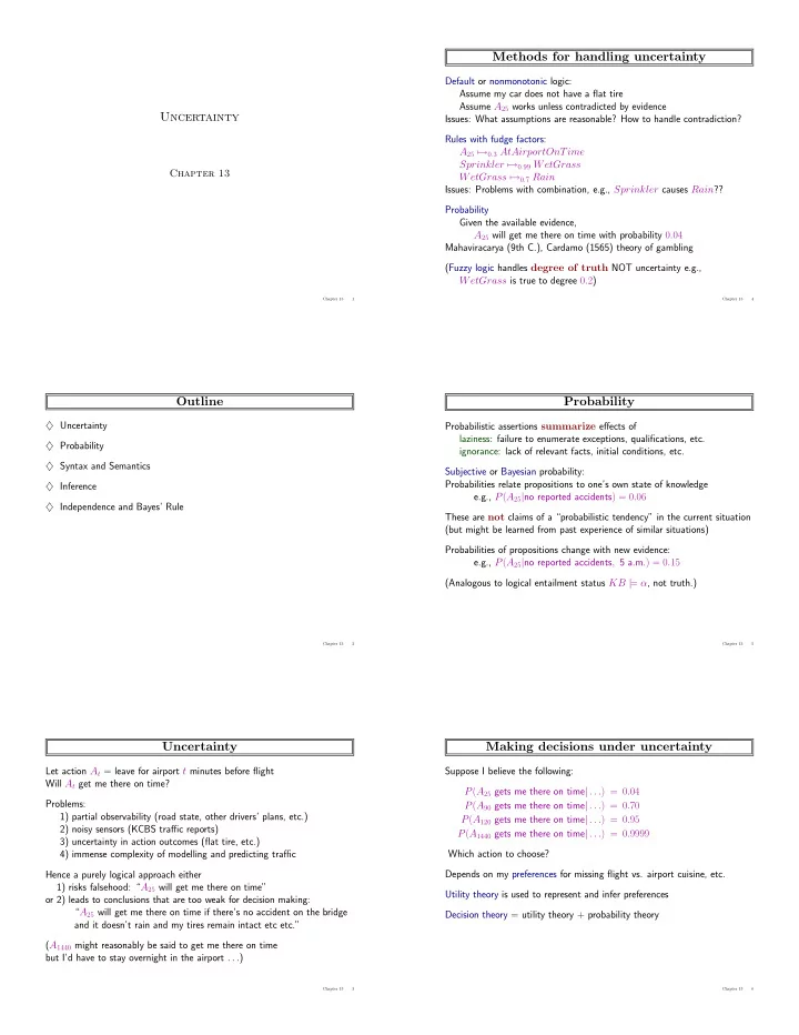
Methods for handling uncertainty Default or nonmonotonic logic: Assume my car does not have a flat tire Assume A 25 works unless contradicted by evidence Uncertainty Issues: What assumptions are reasonable? How to handle contradiction? Rules

SLIDE 1

Uncertainty

Chapter 13

Chapter 13 1

Outline

♦ Uncertainty ♦ Probability ♦ Syntax and Semantics ♦ Inference ♦ Independence and Bayes’ Rule

Chapter 13 2

Uncertainty

Let action At = leave for airport t minutes before flight Will At get me there on time? Problems: 1) partial observability (road state, other drivers’ plans, etc.) 2) noisy sensors (KCBS traffic reports) 3) uncertainty in action outcomes (flat tire, etc.) 4) immense complexity of modelling and predicting traffic Hence a purely logical approach either 1) risks falsehood: “A25 will get me there on time”

r 2) leads to conclusions that are too weak for decision making:

“A25 will get me there on time if there’s no accident on the bridge and it doesn’t rain and my tires remain intact etc etc.” (A1440 might reasonably be said to get me there on time but I’d have to stay overnight in the airport . . .)

Chapter 13 3

Methods for handling uncertainty

Default or nonmonotonic logic: Assume my car does not have a flat tire Assume A25 works unless contradicted by evidence Issues: What assumptions are reasonable? How to handle contradiction? Rules with fudge factors: A25 →0.3 AtAirportOnTime Sprinkler →0.99 WetGrass WetGrass →0.7 Rain Issues: Problems with combination, e.g., Sprinkler causes Rain?? Probability Given the available evidence, A25 will get me there on time with probability 0.04 Mahaviracarya (9th C.), Cardamo (1565) theory of gambling (Fuzzy logic handles degree of truth NOT uncertainty e.g., WetGrass is true to degree 0.2)

Chapter 13 4

Probability

Probabilistic assertions summarize effects of laziness: failure to enumerate exceptions, qualifications, etc. ignorance: lack of relevant facts, initial conditions, etc. Subjective or Bayesian probability: Probabilities relate propositions to one’s own state of knowledge e.g., P(A25|no reported accidents) = 0.06 These are not claims of a “probabilistic tendency” in the current situation (but might be learned from past experience of similar situations) Probabilities of propositions change with new evidence: e.g., P(A25|no reported accidents, 5 a.m.) = 0.15 (Analogous to logical entailment status KB | = α, not truth.)

Chapter 13 5

Making decisions under uncertainty

Suppose I believe the following: P(A25 gets me there on time| . . .) = 0.04 P(A90 gets me there on time| . . .) = 0.70 P(A120 gets me there on time| . . .) = 0.95 P(A1440 gets me there on time| . . .) = 0.9999 Which action to choose? Depends on my preferences for missing flight vs. airport cuisine, etc. Utility theory is used to represent and infer preferences Decision theory = utility theory + probability theory

Chapter 13 6

SLIDE 2

Probability basics

Begin with a set Ω—the sample space e.g., 6 possible rolls of a die. ω ∈ Ω is a sample point/possible world/atomic event A probability space or probability model is a sample space with an assignment P(ω) for every ω ∈ Ω s.t. 0 ≤ P(ω) ≤ 1

ΣωP(ω) = 1

e.g., P(1) = P(2) = P(3) = P(4) = P(5) = P(6) = 1/6. An event A is any subset of Ω P(A) = Σ{ω∈A}P(ω) E.g., P(die roll < 4) = P(1) + P(2) + P(3) = 1/6 + 1/6 + 1/6 = 1/2

Chapter 13 7

Random variables

A random variable is a function from sample points to some range, e.g., the reals or Booleans e.g., Odd(1) = true. P induces a probability distribution for any r.v. X: P(X = xi) = Σ{ω:X(ω) = xi}P(ω) e.g., P(Odd = true) = P(1) + P(3) + P(5) = 1/6 + 1/6 + 1/6 = 1/2

Chapter 13 8

Propositions

Think of a proposition as the event (set of sample points) where the proposition is true Given Boolean random variables A and B: event a = set of sample points where A(ω) = true event ¬a = set of sample points where A(ω) = false event a ∧ b = points where A(ω) = true and B(ω) = true Often in AI applications, the sample points are defined by the values of a set of random variables, i.e., the sample space is the Cartesian product of the ranges of the variables With Boolean variables, sample point = propositional logic model e.g., A = true, B = false, or a ∧ ¬b. Proposition = disjunction of atomic events in which it is true e.g., (a ∨ b) ≡ (¬a ∧ b) ∨ (a ∧ ¬b) ∨ (a ∧ b) ⇒ P(a ∨ b) = P(¬a ∧ b) + P(a ∧ ¬b) + P(a ∧ b)

Chapter 13 9

Why use probability?

The definitions imply that certain logically related events must have related probabilities E.g., P(a ∨ b) = P(a) + P(b) − P(a ∧ b)

A B True A B

de Finetti (1931): an agent who bets according to probabilities that violate these axioms can be forced to bet so as to lose money regardless of outcome.

Chapter 13 10

Syntax for propositions

Propositional or Boolean random variables e.g., Cavity (do I have a cavity?) Cavity = true is a proposition, also written cavity Discrete random variables (finite or infinite) e.g., Weather is one of sunny, rain, cloudy, snow Weather = rain is a proposition Values must be exhaustive and mutually exclusive Continuous random variables (bounded or unbounded) e.g., Temp = 21.6; also allow, e.g., Temp < 22.0. Arbitrary Boolean combinations of basic propositions

Chapter 13 11

Prior probability

Prior or unconditional probabilities of propositions e.g., P(Cavity = true) = 0.1 and P(Weather = sunny) = 0.72 correspond to belief prior to arrival of any (new) evidence Probability distribution gives values for all possible assignments: P(Weather) = 0.72, 0.1, 0.08, 0.1 (normalized, i.e., sums to 1) Joint probability distribution for a set of r.v.s gives the probability of every atomic event on those r.v.s (i.e., every sample point) P(Weather, Cavity) = a 4 × 2 matrix of values: Weather = sunny rain cloudy snow Cavity = true 0.144 0.02 0.016 0.02 Cavity = false 0.576 0.08 0.064 0.08 Every question about a domain can be answered by the joint distribution because every event is a sum of sample points

Chapter 13 12

SLIDE 3

Probability for continuous variables

Express distribution as a parameterized function of value: P(X = x) = U[18, 26](x) = uniform density between 18 and 26 0.125 dx 18 26 Here P is a density; integrates to 1. P(X = 20.5) = 0.125 really means lim

dx→0 P(20.5 ≤ X ≤ 20.5 + dx)/dx = 0.125

Chapter 13 13

Gaussian density

P(x) =

1 √ 2πσe−(x−µ)2/2σ2

Chapter 13 14

Conditional probability

Conditional or posterior probabilities e.g., P(cavity|toothache) = 0.8 i.e., given that toothache is all I know NOT “if toothache then 80% chance of cavity” (Notation for conditional distributions: P(Cavity|Toothache) = 2-element vector of 2-element vectors) If we know more, e.g., cavity is also given, then we have P(cavity|toothache, cavity) = 1 Note: the less specific belief remains valid after more evidence arrives, but is not always useful New evidence may be irrelevant, allowing simplification, e.g., P(cavity|toothache,49ersWin) = P(cavity|toothache) = 0.8 This kind of inference, sanctioned by domain knowledge, is crucial

Chapter 13 15

Conditional probability

Definition of conditional probability: P(a|b) = P(a ∧ b) P(b) if P(b) = 0 Product rule gives an alternative formulation: P(a ∧ b) = P(a|b)P(b) = P(b|a)P(a) A general version holds for whole distributions, e.g., P(Weather, Cavity) = P(Weather|Cavity)P(Cavity) (View as a 4 × 2 set of equations, not matrix mult.) Chain rule is derived by successive application of product rule: P(X1, . . . , Xn) = P(X1, . . . , Xn−1) P(Xn|X1, . . . , Xn−1) = P(X1, . . . , Xn−2) P(Xn1|X1, . . . , Xn−2) P(Xn|X1, . . . , Xn−1) = . . . = Πn

i = 1P(Xi|X1, . . . , Xi−1)

Chapter 13 16

Inference by enumeration

Start with the joint distribution:

cavity

toothache cavity catch catch

toothache

catch catch

.108 .012 .016 .064 .072 .144 .008 .576

For any proposition φ, sum the atomic events where it is true: P(φ) = Σω:ω|

=φP(ω)

Chapter 13 17

Inference by enumeration

Start with the joint distribution:

cavity

toothache cavity catch catch

toothache

catch catch

.108 .012 .016 .064 .072 .144 .008 .576

For any proposition φ, sum the atomic events where it is true: P(φ) = Σω:ω|

=φP(ω)

P(toothache) = 0.108 + 0.012 + 0.016 + 0.064 = 0.2

Chapter 13 18

SLIDE 4

Inference by enumeration

Start with the joint distribution:

cavity

toothache cavity catch catch

toothache

catch catch

.108 .012 .016 .064 .072 .144 .008 .576

For any proposition φ, sum the atomic events where it is true: P(φ) = Σω:ω|

=φP(ω)

P(cavity∨toothache) = 0.108+0.012+0.072+0.008+0.016+0.064 = 0.28

Chapter 13 19

Inference by enumeration

Start with the joint distribution:

cavity

toothache cavity catch catch

toothache

catch catch

.108 .012 .016 .064 .072 .144 .008 .576

Can also compute conditional probabilities: P(¬cavity|toothache) = P(¬cavity ∧ toothache) P(toothache) = 0.016 + 0.064 0.108 + 0.012 + 0.016 + 0.064 = 0.4

Chapter 13 20

Normalization

cavity

toothache cavity catch catch

toothache

catch catch

.108 .012 .016 .064 .072 .144 .008 .576

Denominator can be viewed as a normalization constant α P(Cavity|toothache) = α P(Cavity, toothache) = α [P(Cavity, toothache, catch) + P(Cavity, toothache, ¬catch)] = α [0.108, 0.016 + 0.012, 0.064] = α 0.12, 0.08 = 0.6, 0.4 General idea: compute distribution on query variable by fixing evidence variables and summing over hidden variables

Chapter 13 21

Inference by enumeration, contd.

Let X be all the variables. Typically, we want the posterior joint distribution of the query variables Y given specific values e for the evidence variables E Let the hidden variables be H = X − Y − E Then the required summation of joint entries is done by summing out the hidden variables: P(Y|E = e) = αP(Y, E = e) = αΣhP(Y, E = e, H = h) The terms in the summation are joint entries because Y, E, and H together exhaust the set of random variables Obvious problems: 1) Worst-case time complexity O(dn) where d is the largest arity 2) Space complexity O(dn) to store the joint distribution 3) How to find the numbers for O(dn) entries???

Chapter 13 22

Independence

A and B are independent iff P(A|B) = P(A)

P(B|A) = P(B)

P(A, B) = P(A)P(B)

Weather Toothache Catch Cavity

decomposes into

Weather Toothache Catch Cavity

P(Toothache, Catch, Cavity, Weather) = P(Toothache, Catch, Cavity)P(Weather) 32 entries reduced to 12; for n independent biased coins, 2n → n Absolute independence powerful but rare Dentistry is a large field with hundreds of variables, none of which are independent. What to do?

Chapter 13 23

Conditional independence

P(Toothache, Cavity, Catch) has 23 − 1 = 7 independent entries If I have a cavity, the probability that the probe catches in it doesn’t depend

n whether I have a toothache:

Chapter 13 24

SLIDE 5

Conditional independence contd.

Write out full joint distribution using chain rule: P(Toothache, Catch, Cavity) = P(Toothache|Catch, Cavity)P(Catch, Cavity) = P(Toothache|Catch, Cavity)P(Catch|Cavity)P(Cavity) = P(Toothache|Cavity)P(Catch|Cavity)P(Cavity) I.e., 2 + 2 + 1 = 5 independent numbers (equations 1 and 2 remove 2) In most cases, the use of conditional independence reduces the size of the representation of the joint distribution from exponential in n to linear in n. Conditional independence is our most basic and robust form of knowledge about uncertain environments.

Chapter 13 25

Bayes’ Rule

Product rule P(a ∧ b) = P(a|b)P(b) = P(b|a)P(a) ⇒ Bayes’ rule P(a|b) = P(b|a)P(a) P(b)

r in distribution form

Chapter 13 26

Bayes’ Rule and conditional independence

Toothache Cavity Catch Cause Effect1 Effectn

Total number of parameters is linear in n

Chapter 13 27

Wumpus World

1,1 2,1 3,1 4,1 1,2 2,2 3,2 4,2 1,3 2,3 3,3 4,3 1,4 2,4

OK OK

3,4 4,4

B B

Pij = true iff [i, j] contains a pit Bij = true iff [i, j] is breezy Include only B1,1, B1,2, B2,1 in the probability model

Chapter 13 28

Specifying the probability model

The full joint distribution is P(P1,1, . . . , P4,4, B1,1, B1,2, B2,1) Apply product rule: P(B1,1, B1,2, B2,1 | P1,1, . . . , P4,4)P(P1,1, . . . , P4,4) (Do it this way to get P(Effect|Cause).) First term: 1 if pits are adjacent to breezes, 0 otherwise Second term: pits are placed randomly, probability 0.2 per square: P(P1,1, . . . , P4,4) = Π4,4

i,j = 1,1P(Pi,j) = 0.2n × 0.816−n

for n pits.

Chapter 13 29

Observations and query

We know the following facts: b = ¬b1,1 ∧ b1,2 ∧ b2,1 known = ¬p1,1 ∧ ¬p1,2 ∧ ¬p2,1 Query is P(P1,3|known, b) Define Unknown = Pijs other than P1,3 and Known For inference by enumeration, we have P(P1,3|known, b) = αΣunknownP(P1,3, unknown, known, b) Grows exponentially with number of squares!

Chapter 13 30

SLIDE 6

Using conditional independence

Basic insight: observations are conditionally independent of other hidden squares given neighbouring hidden squares

1,1 2,1 3,1 4,1 1,2 2,2 3,2 4,2 1,3 2,3 3,3 4,3 1,4 2,4 3,4 4,4 KNOWN FRINGE QUERY OTHER

Define Unknown = Fringe ∪ Other P(b|P1,3, Known, Unknown) = P(b|P1,3, Known, Fringe) Manipulate query into a form where we can use this!

Chapter 13 31

Using conditional independence contd.

P(P1,3|known, b) = α

unknown P(P1,3, unknown, known, b)

= α

unknown P(b|P1,3, known, unknown)P(P1,3, known, unknown)

= α

fringe
ther P(b|known, P1,3, fringe, other)P(P1,3, known, fringe, other)

= α

fringe
ther P(b|known, P1,3, fringe)P(P1,3, known, fringe, other)

= α

fringeP(b|known, P1,3, fringe)
therP(P1,3, known, fringe, other)

= α

fringe P(b|known, P1,3, fringe)
ther P(P1,3)P(known)P(fringe)P(other)

= α P(known)P(P1,3)

fringe P(b|known, P1,3, fringe)P(fringe)
ther P(other)

= α′ P(P1,3)

fringe P(b|known, P1,3, fringe)P(fringe)

Chapter 13 32

Using conditional independence contd.

OK 1,1 2,1 3,1 1,2 2,2 1,3 OK OK B B OK 1,1 2,1 3,1 1,2 2,2 1,3 OK OK B B OK 1,1 2,1 3,1 1,2 2,2 1,3 OK OK B B

0.2 x 0.2 = 0.04 0.2 x 0.8 = 0.16 0.8 x 0.2 = 0.16

OK 1,1 2,1 3,1 1,2 2,2 1,3 OK OK B B OK 1,1 2,1 3,1 1,2 2,2 1,3 OK OK B B

0.2 x 0.2 = 0.04 0.2 x 0.8 = 0.16

P(P1,3|known, b) = α′ 0.2(0.04 + 0.16 + 0.16), 0.8(0.04 + 0.16) ≈ 0.31, 0.69 P(P2,2|known, b) ≈ 0.86, 0.14

Chapter 13 33

Summary

Probability is a rigorous formalism for uncertain knowledge Joint probability distribution specifies probability of every atomic event Queries can be answered by summing over atomic events For nontrivial domains, we must find a way to reduce the joint size Independence and conditional independence provide the tools

Chapter 13 34