MergeSort [5] In the last class Insertion sort Analysis of - PDF document

Algorithm : Design & Analysis MergeSort [5]

In the last class… � Insertion sort � Analysis of insertion sorting algorithm � Lower bound of local comparison based sorting algorithm � General pattern of divide-and-conquer � Quicksort � Analysis of Quicksort

Mergesort � Mergesort � Worst Case Analysis of Mergesort � Lower Bounds for Sorting by Comparison of Keys � Worst Case � Average Behavior

MergeSort: the Strategy � Easy division � No comparison is done during the division � Minimizing the size difference between the divided subproblems � Merging two sorted subranges � Using Merge

Merging Sorted Arrays indexA indexB A[ k -1] A[0] B[0] B[ m -1] B A Comparing MIN C Space to be filled Sorted elements Never examined again indexC

Merge: the Specification � Input: Array A with k elements and B with m elements, each in nondecreasing order of their key. � Output: C , an array containing n = k + m elements from A and B in nondecreasing order. C is passed in and the algorithm fills it.

Merge: the Recursive Version merge( A , B , C ) Base cases if ( A is empty) rest of C = rest of B else if ( B is empty) rest of C = rest of A else if (first of A ≤ first of B ) first of C =first of A merge(rest of A , B , rest of C ) else first of C =first of B merge(A, rest of B, rest of C) return

Worst Case Complexity of Merge � Observations: � After each comparison, one element is inserted into Array C, at least . � After entering Array C, an element will never be compared again � After the last comparison, at least two elements have not yet been moved to Array C. So at most n -1 comparisons are done. � Worst case is that the last comparison is conducted between A[ k -1] and B[ m -1] � In worst case, n-1 comparisons are done, where n = k + m

Optimality of Merge � Any algorithm to merge two sorted arrays, each containing k = m = n /2 entries, by comparison of keys, does at least n -1 comparisons in the worst case. � Choose keys so that: b 0 <a 0 <b 1 < a 1 <...< b i < a i < b i+1 ,...,< b m-1 < a k-1 � Then the algorithm must compare a i with b i for every i in [0, m -1], and must compare a i with b i+1 for every i in [0, m -2], so, there are n -1 comparisons. Valid for | k - m | ≤ 1, as well.

Space Complexity of Merge � A algorithm is “in space”, if the extra space it has to use is in Θ (1) � Merge is not a algorithm “in space”, since it need enough extra space to store the merged sequence during the merging process.

Overlapping Arrays for Merge extra space Before the merge 0 m -1 k+m -1 0 k -1 B A Merge from the right Partly finished Merged 0 m -1 k+m -1 0 k -1 0 m -1 k+m -1 0 k -1 A/C Finished

MergeSort � Input: Array E and indexes first , and last , such that the elements of E [ i ] are defined for first ≤ i ≤ last . � Output: E[ first ],…,E[ last ] is a sorted rearrangement of the same elements. � Procedure void mergeSort(Element[] E, int first, int last) if (first<last) int mid=(first+last)/2; mergeSort(E, first, mid); mergeSort(E, mid+1, last); merge(E, first, mid, last) return

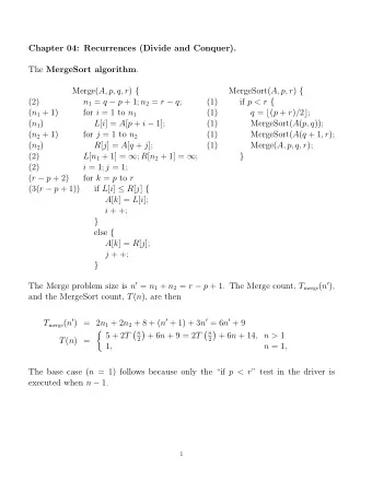
Analysis of Mergesort � The recurrence equation for Mergesort � W(n)=W( ⎣ n/2 ⎦ )+W( ⎡ n/2 ⎤ )+n-1 � W(1)=0 Where n =last-first+1, the size of range to be sorted � The Master Theorem applies for the equation, so: W ( n ) ∈ Θ ( n log n )

Recursion Tree for Mergesort n-1 Level 0 Base cases occur at depth ⎡ lg(n+1) ⎤ -1 Level 1 n-2 and ⎡ lg(n+1) ⎤ Level 2 n-4 n-8 Level 3 Note: nonrecursive costs on level k is n -2 k for T(n) n-1 n/2-1 T(n/2) all level without k /2 may be basecase node ⎡ k /2 ⎤ or ⎣ k /2 ⎦ n/8-1 T(n/8) T(n/4) n/4-1

Non-complete Recursive Tree Example: n=11 2 D -1 nodes B base-case nodes on the second lowest level Since each nonbase-case n - B base-case nodes node has 2 children, there No nonbase-case nodes at this depth are ( n - B )/2 nonbase-case nodes at depth D -1

Number of Comparison of Mergesort The maximum depth D of the recursive tree is ⎡ lg(n+1) ⎤ . � Let B base case nodes on depth D -1, and n - B on depth D, (Note: base case � node has nonrecursive cost 0). ( n - B )/2 nonbase case nodes at depth D -1, each has nonrecursive cost 1. � So: � − = ∑ 2 D − − n B n B − − + = − − 1 − + d D ( ) ( 2 ) ( 1 ) ( 2 1 ) W n n n D 2 2 = 0 d − + = = − D D ( 2 2 ) , 2 Since B B n that is B n = − + D , ( ) 2 1 So W n nD D 2 B = + = α ≤ α < = + α 1 , 1 2 , lg lg Let then D n n n = − α − α + , ( ) lg ( lg ) 1 So W n n n n ⎡ nlg(n)-n+1 ⎤ ≤ number of comparison ≤ ⎡ nlg(n)-0.914n ⎤ �

Decision Tree for Sorting Internal node Internal node 1:2 A example for n=3 2:3 1:3 x 2 , x 1 , x 3 1:3 x 1 , x 2 , x 3 2:3 External node x 3 , x 2 , x 1 x 3 , x 1 , x 2 x 2 , x 3 , x 1 External node x 1 , x 3 , x 2 � Decision tree is a 2-tree.(Assuming no same keys) � The action of Sort on a particular input corresponds to following on path in its decision tree from the root to a leaf associated to the specific output

Characteristics of the Decision Tree � For a sequence of n distinct elements, there are n! different permutation, so, the decision tree has at least n! leaves, and exactly n! leaves can be reached from the root. So, for the purpose of lower bounds evaluation, we use trees with exactly n! leaves. � The number of comparison done in the worst case is the height of the tree. � The average number of comparison done is the average of the lengths of all paths from the root to a leaf.

Lower Bound for Worst Case � Theorem : Any algorithm to sort n items by comparisons of keys must do at least ⎡ lg n ! ⎤ , or approximately ⎡ n lg n -1.443 n ⎤ , key comparisons in the worst case. � Note: Let L= n !, which is the number of leaves, then L ≤ 2 h , where h is the height of the tree, that is h ≥ ⎡ lg L ⎤ = ⎡ lg n ! ⎤ � For the asymptotic behavior: n ⎛ ⎞ ⎡ ⎤ ⎛ ⎞ ⎛ ⎞ n n n n 2 ⎜ ⎟ ≥ − ≥ = ∈ Θ ⎜ ⎟ ⎜ ⎟ lg( ! ) lg[ ( 1 )... ] lg lg ( lg ) n n n n n ⎜ ⎢ ⎥ ⎟ ⎢ ⎥ ⎝ ⎠ ⎝ ⎠ ⎝ 2 ⎠ 2 2 2 derived using: n ∑ = lg ! lg( ) n j = 1 j

2-Tree � 2-Tree � Common Binary Tree internal nodes Both left and right external nodes children of these no child nodes are empty tree any type

External Path Length(EPL) � The EPL of a 2-tree t is defined as follows: � [Base case] 0 for a single external node � [Recursion] t is non-leaf with sub-trees L and R , then the sum of: � the external path length of L ; � the number of external node of L ; � the external path length of R ; � the number of external node of R ;

Properties of EPL � Let t is a 2-tree, then the epl of t is the sum of the paths from the root to each external node. � epl ≥ m lg( m ), where m is the number of external nodes in t � epl=epl L +epl R +m ≥ m L lg( m L )+ m R lg( m R )+ m , � note f (x)+ f (y) ≥ 2 f ((x+y)/2) for f( x )= x lg x � so, epl ≥ 2(( m L + m R )/2)lg(( m L + m R )/2)+ m = m (lg( m )-1)+ m = m lg m .

Lower Bound for Average Behavior � Since a decision tree with L leaves is a 2-tree, the epl average path length from the root to a leaf is . L � The trees that minimize epl are as balanced as possible. to be proved � Recall that epl ≥ L lg( L ). � Theorem : The average number of comparison done by an algorithm to sort n items by comparison of keys is at least lg( n !), which is about n lg n -1.443 n .

Reducing External Path Length X level k X level k +1 Y level h -1 Y level h Assuming that h - k >1, when calculating epl , h + h + k is replaced by ( h -1)+2( k +1). The net change in epl is k - h +1<0, that is, the epl decreases. So, more balanced 2-tree has smaller epl.

Mergesort Has Optimal Average Performance � We have proved that the average number of comparisons done by an algorithm to sort n items by comparison of keys is at least about n lg n -1.443 n � The worst complexity of mergesort is in Θ ( n lg n ) � But, the average performance can not be worse the the worst case performance. � So, mergesort is optimal as for its average performance.

Home Assignment � pp.212- � 4.24 � 4.25 � 4.27 � 4.29 � 4.30 � 4.32