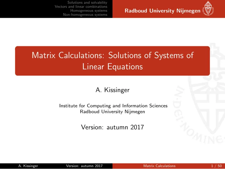
[PPT] - Matrix Calculations: Solutions of Systems of Linear Equations A. PowerPoint Presentation

SLIDE 1

Solutions and solvability Vectors and linear combinations Homogeneous systems Non-homogeneous systems

Radboud University Nijmegen

Matrix Calculations: Solutions of Systems of Linear Equations

A. Kissinger

Institute for Computing and Information Sciences Radboud University Nijmegen

Version: autumn 2017

A. Kissinger

Version: autumn 2017 Matrix Calculations 1 / 50

SLIDE 2

Solutions and solvability Vectors and linear combinations Homogeneous systems Non-homogeneous systems

Radboud University Nijmegen

Outline

Solutions and solvability Vectors and linear combinations Homogeneous systems Non-homogeneous systems

A. Kissinger

Version: autumn 2017 Matrix Calculations 2 / 50

SLIDE 3

Solutions and solvability Vectors and linear combinations Homogeneous systems Non-homogeneous systems

Radboud University Nijmegen

Solutions

When we look for solutions to a system, there are 3 possibilities:

1 A system of equations has a single, unique solution, e.g.

x1 + x2 = 3 x1 − x2 = 1

(unique solution: x1 = 2, x2 = 1)

2 A system has many solutions, e.g.

x1 − 2x2 = 1 −2x1 + 4x2 = −2

(we have a solution whenever: x1 = 1 + 2x2)

3 A system has no solutions.

3x1 − 2x2 = 1 6x1 − 4x2 = 6

(the transformation E2 := E2 − 2E1 yields 0 = 4.)

A. Kissinger

Version: autumn 2017 Matrix Calculations 4 / 50

SLIDE 4

Solutions and solvability Vectors and linear combinations Homogeneous systems Non-homogeneous systems

Radboud University Nijmegen

Solutions, geometrically

Consider systems of only two variables x, y. A linear equation ax + by = c then describes a line in the plane. For 2 such equations/lines, there are three possibilities:

1 the lines intersect in a unique point, which is the solution to

both equations

2 the lines are parallel, in which case there are no joint solutions 3 the lines coincide, giving many joint solutions.

A. Kissinger

Version: autumn 2017 Matrix Calculations 5 / 50

SLIDE 5

Solutions and solvability Vectors and linear combinations Homogeneous systems Non-homogeneous systems

Radboud University Nijmegen

Echelon form

We can tell the difference in these 3 cases by writing the augmented matrix and tranforming to Echelon form. Recall: A matrix is in Echelon form if:

1 All of the rows with pivots occur before zero rows, and 2 Pivots always occur to the right of previous pivots

     3 2 5 −5 1 2 1 −2

2

2     

A. Kissinger

Version: autumn 2017 Matrix Calculations 6 / 50

SLIDE 6

Solutions and solvability Vectors and linear combinations Homogeneous systems Non-homogeneous systems

Radboud University Nijmegen

(In)consistent systems

Definition

A system of equations is consistent (oplosbaar) if it has one or more solutions. Otherwise, when there are no solutions, the system is called inconsistent Thus, for a system of equations:

nr. of solutions

terminology inconsistent ≥ 1

(one or many)

consistent

A. Kissinger

Version: autumn 2017 Matrix Calculations 7 / 50

SLIDE 7

Solutions and solvability Vectors and linear combinations Homogeneous systems Non-homogeneous systems

Radboud University Nijmegen

Inconsistency and echelon forms

Theorem

A system of equations is inconsistent (non-solvable) if and only if in the echelon form of its augmented matrix there is a row with:

only zeros before the bar |
a non-zero after the bar |,

as in: 0 0 · · · 0 | c, where c = 0.

Example

3x1 − 2x2 = 1 6x1 − 4x2 = 6 gives 3 −2 1 6 −4 6

and

3 −2 1 4

(using the transformation R2 := R2 − 2R1)
A. Kissinger

Version: autumn 2017 Matrix Calculations 8 / 50

SLIDE 8

Solutions and solvability Vectors and linear combinations Homogeneous systems Non-homogeneous systems

Radboud University Nijmegen

Unique solutions

Theorem

A system of equations in n variables has a unique solution if and

nly if in its Echelon form there are n pivots.
Proof. (n pivots =

⇒ unique soln., on board)

In summary: A system with n variables has an augmented matrix with n columns before the line. Its Echelon form has n pivots, so there must be exactly one pivot in each column. The last pivot uniquely fixes xn. Then, since xn is fixed, the second to last pivot uniquely fixes xn−1 and so on.

A. Kissinger

Version: autumn 2017 Matrix Calculations 9 / 50

SLIDE 9

Solutions and solvability Vectors and linear combinations Homogeneous systems Non-homogeneous systems

Radboud University Nijmegen

Unique solutions: earlier example

equations matrix 2x2 + x3 = −2 3x1 + 5x2 − 5x3 = 1 2x1 + 4x2 − 2x3 = 2   0 2 1 −2 3 5 −5 1 2 4 −2 2   After various transformations leads to x1 + 2x2 − 1x3 = 1 x2 + 2x3 = 2 x3 = 2   1 2 −1 1 0 1 2 2 0 0 1 2  

☛ ✡ ✟ ✠

Echelon form There are 3 variables and 3 pivots, so there is one unique solution.

A. Kissinger

Version: autumn 2017 Matrix Calculations 10 / 50

SLIDE 10

Solutions and solvability Vectors and linear combinations Homogeneous systems Non-homogeneous systems

Radboud University Nijmegen

Unique solutions

So, when there are n pivots, there is 1 solution, and life is good. Question: What if there are more solutions? Can we describe them in a generic way?

A. Kissinger

Version: autumn 2017 Matrix Calculations 11 / 50

SLIDE 11

Solutions and solvability Vectors and linear combinations Homogeneous systems Non-homogeneous systems

Radboud University Nijmegen

A new tool: vectors

A vector is a list of numbers.
We can write it like this: (x1, x2, . . . , xn)
...or as a matrix with just one column:

     x1 x2 . . . xn      (which is sometimes called a ‘column vector’).

A. Kissinger

Version: autumn 2017 Matrix Calculations 13 / 50

SLIDE 12

Solutions and solvability Vectors and linear combinations Homogeneous systems Non-homogeneous systems

Radboud University Nijmegen

A new tool: vectors

Vectors are useful for lots of stuff. In this lecture, we’ll use

them to hold solutions.

Since variable names don’t matter, we can write this:

x1 := 2 x2 := −1 x3 := 0

...more compactly as this:

  2 −1  

...or even more compactly as this: (2, −1, 0).
A. Kissinger

Version: autumn 2017 Matrix Calculations 14 / 50

SLIDE 13

Solutions and solvability Vectors and linear combinations Homogeneous systems Non-homogeneous systems

Radboud University Nijmegen

Linear combinations

We can multiply a vector by a number to get a new vector:

c ·      x1 x2 . . . xn      :=      cx1 cx2 . . . cxn      This is called scalar multiplication.

...and we can add vectors together:

     x1 x2 . . . xn      +      y1 y2 . . . yn      :=      x1 + y1 x2 + y2 . . . xn + yn      as long as the are the same length.

A. Kissinger

Version: autumn 2017 Matrix Calculations 15 / 50

SLIDE 14

Solutions and solvability Vectors and linear combinations Homogeneous systems Non-homogeneous systems

Radboud University Nijmegen

Linear combinations

Mixing these two things together gives us a linear combination of vectors: c ·      x1 x2 . . . xn      + d ·      y1 y2 . . . yn      + . . . =      cx1 + dy1 + . . . cx2 + dy2 + . . . . . . cxn + dyn + . . .      A set of vectors v1, v2, . . . , vk is called linearly independent if no vector can be written as a linear combination of the others.

A. Kissinger

Version: autumn 2017 Matrix Calculations 16 / 50

SLIDE 15

Solutions and solvability Vectors and linear combinations Homogeneous systems Non-homogeneous systems

Radboud University Nijmegen

Linear independence

These vectors:

v1 = 1

v2 =

1

v3 =

1 1

are NOT linearly independent, because v3 = v1 + v2.
These vectors:

v1 =   1 2 3   v2 =   1 1   v3 =   1 1   are NOT linearly independent, because v1 = v2 + 2 · v3.

A. Kissinger

Version: autumn 2017 Matrix Calculations 17 / 50

SLIDE 16

Solutions and solvability Vectors and linear combinations Homogeneous systems Non-homogeneous systems

Radboud University Nijmegen

Linear independence

These vectors:

v1 =   1   v2 =   1   v3 =   1   are linearly independent. There is no way to write any of them in terms of each other.

These vectors:

v1 =   1   v2 =   1   v3 =   2 2   are linearly independent. There is no way to write any of them in terms of each other.

A. Kissinger

Version: autumn 2017 Matrix Calculations 18 / 50

SLIDE 17

Solutions and solvability Vectors and linear combinations Homogeneous systems Non-homogeneous systems

Radboud University Nijmegen

Linear independence

These vectors:

v1 =   1 2 3   v2 =   2 −1 4   v3 =   5 2   are... ???

‘Eyeballing’ vectors works sometimes, but we need a better

way of checking linear independence!

A. Kissinger

Version: autumn 2017 Matrix Calculations 19 / 50

SLIDE 18

Solutions and solvability Vectors and linear combinations Homogeneous systems Non-homogeneous systems

Radboud University Nijmegen

Checking linear independence

Theorem

Vectors v1, . . . , vn are linearly independent if and only if, for all numbers a1, . . . , an ∈ R one has: a1 · v1 + · · · + an · vn = 0 implies a1 = a2 = · · · = an = 0

Example

The 3 vectors (1, 0, 0), (0, 1, 0), (0, 0, 1) are linearly independent, since if a1 · (1, 0, 0) + a2 · (0, 1, 0) + a3 · (0, 0, 1) = (0, 0, 0) then, using the computation from the previous slide, (a1, a2, a3) = (0, 0, 0), so that a1 = a2 = a3 = 0

A. Kissinger

Version: autumn 2017 Matrix Calculations 20 / 50

SLIDE 19

Solutions and solvability Vectors and linear combinations Homogeneous systems Non-homogeneous systems

Radboud University Nijmegen

Checking linear independence

Theorem

Vectors v1, . . . , vn are linearly independent if and only if, for all numbers a1, . . . , an ∈ R one has: a1 · v1 + · · · + an · vn = 0 implies a1 = a2 = · · · = an = 0

Proof. Another way to say the theorem is v1, . . . , vn are linearly

dependent if and only if: a1 · v1 + a2 · v2 + · · · + an · vn = 0 where some aj are non-zero. If this is true and a1 = 0, then: v1 = (−a2/a1) · v2 + . . . + (−an/a1) · vn The vectors are dependent (also works for any other non-zero aj). Exercise: prove the other direction.

A. Kissinger

Version: autumn 2017 Matrix Calculations 21 / 50

SLIDE 20

Solutions and solvability Vectors and linear combinations Homogeneous systems Non-homogeneous systems

Radboud University Nijmegen

Proving (in)dependence via equation solving I

Investigate (in)dependence of

  1 2 3  ,   2 −1 4  , and   5 2  

Thus we ask: are there any non-zero a1, a2, a3 ∈ R with:

a1   1 2 3   + a2   2 −1 4   + a3   5 2   =    

If there is a non-zero solution, the vectors are dependent, and

if a1 = a2 = a3 = 0 is the only solution, they are independent

A. Kissinger

Version: autumn 2017 Matrix Calculations 22 / 50

SLIDE 21

Solutions and solvability Vectors and linear combinations Homogeneous systems Non-homogeneous systems

Radboud University Nijmegen

Proving (in)dependence via equation solving II

Our question involves the systems of equations / matrix:

   a1 + 2a2 = 0 2a1 − a2 + 5a3 = 0 3a1 + 4a2 + 2a3 = 0 corresponding to   1 2 0 −1 1   (in Echelon form)

This has only 2 pivots, so multiple solutions. In particular, it

has non-zero solutions, for example: a1 = 2, a2 = −1, a3 = −1

(compute and check for yourself!)

Thus the original vectors are dependent. Explicitly:

2   1 2 3   + (−1)   2 −1 4   + (−1)   5 2   =    

A. Kissinger

Version: autumn 2017 Matrix Calculations 23 / 50

SLIDE 22

Solutions and solvability Vectors and linear combinations Homogeneous systems Non-homogeneous systems

Radboud University Nijmegen

Proving (in)dependence via equation solving III

Same (in)dependence question for:

  1 2 −3  ,   −2 1 1  ,   1 −1 −2  

With corresponding matrix:

  1 −2 1 2 1 −1 −3 1 −2   reducing to   5 0 −1 0 5 −3 0 0 −4  

Thus the only solution is a1 = a2 = a3 = 0. The vectors are

independent!

A. Kissinger

Version: autumn 2017 Matrix Calculations 24 / 50

SLIDE 23

Solutions and solvability Vectors and linear combinations Homogeneous systems Non-homogeneous systems

Radboud University Nijmegen

Linear independence: summary

To check linear independence of v1, v2, . . . , vn:

1 Write the vectors as the columns of a matrix 2 Convert to Echelon form 3 Count the pivots

(# pivots) = (# columns) means independent
(# pivots) < (# columns) means dependent

4 Non-zero solutions show linear dependence explicitly, e.g.

v1 − 2v2 + v3 = 0 = ⇒ v1 = 2v2 − v3

A. Kissinger

Version: autumn 2017 Matrix Calculations 25 / 50

SLIDE 24

Solutions and solvability Vectors and linear combinations Homogeneous systems Non-homogeneous systems

Radboud University Nijmegen

General solutions

The Goal:

Describe the space of solutions of a system of equations.
In general, there can be infinitely many solutions, but only a

few are actually ‘different enough’ to matter. These are called basic solutions.

Using the basic solutions, we can write down a formula which

gives us any solution: the general solution.

Example (General solution for one equation)

2x1 − x2 = 3 gives x2 = 2x1 − 3 So a general solution (for any c) is: x1 := c x2 := 2c − 3

A. Kissinger

Version: autumn 2017 Matrix Calculations 27 / 50

SLIDE 25

Solutions and solvability Vectors and linear combinations Homogeneous systems Non-homogeneous systems

Radboud University Nijmegen

Linear combinations of solutions

It is not the case in general that linear combinations of

solutions give solutions. For example, consider:

x1 + 2x2 + x3 = 0

x2 + x4 = 2 ↔ 1 2 1 0 0 0 1 0 1 2

This has as solutions:

v1 =     −2 2 −2     , v2 =     −1 1 −1 1     but not v1+v2 =     −3 3 −3 1     , 3·v1, . . .

The problem is this system of equations is not homogeneous,

because the the 2 on the right-hand-side (RHS) of the second equation.

A. Kissinger

Version: autumn 2017 Matrix Calculations 28 / 50

SLIDE 26

Solutions and solvability Vectors and linear combinations Homogeneous systems Non-homogeneous systems

Radboud University Nijmegen

Homogeneous systems of equations

Definition

A system of equations is called homogeneous if it has zeros on the RHS of every equation. Otherwise it is called non-homogeneous.

We can always squash a non-homogeneous system to a

homogeneous one:   0 2 1 −2 3 5 −5 1 0 0 −2 2  



 0 2 1 3 5 −5 0 0 −2  

The solutions will change!
...but they are still related. We’ll see how that works soon.
A. Kissinger

Version: autumn 2017 Matrix Calculations 29 / 50

SLIDE 27

Solutions and solvability Vectors and linear combinations Homogeneous systems Non-homogeneous systems

Radboud University Nijmegen

Zero solution, in homogeneous case

Lemma

Each homogeneous equation has (0, . . . , 0) as solution. Proof: A homogeneous system looks like this a11x1 + · · · + a1nxn = 0 . . . am1x1 + · · · + amnxn = 0 Consider the equation at row i: ai1x1 + · · · + ainxn = 0 Clearly it has as solution x1 = x2 = · · · = xn = 0. This holds for each row i.

A. Kissinger

Version: autumn 2017 Matrix Calculations 30 / 50

SLIDE 28

Solutions and solvability Vectors and linear combinations Homogeneous systems Non-homogeneous systems

Radboud University Nijmegen

Linear combinations of solutions

Theorem

The set of solutions of a homogeneous system is closed under linear combinations (i.e. addition and scalar multiplication of vectors). ...which means:

if (s1, s2, . . . , sn) and (t1, t2, . . . , tn) are solutions, then so is:

(s1 + t1, s2 + t2, . . . , sn + tn), and

if (s1, s2, . . . , sn) is a solution, then so is (c · s1, c · s2, . . . , c · sn)
A. Kissinger

Version: autumn 2017 Matrix Calculations 31 / 50

SLIDE 29

Solutions and solvability Vectors and linear combinations Homogeneous systems Non-homogeneous systems

Radboud University Nijmegen

Example

Consider the homogeneous system

3x1 + 2x2 − x3 = 0 x1 − x2 = 0

A solution is x1 = 1, x2 = 1, x3 = 5, written as vector

(x1, x2, x3) = (1, 1, 5)

Another solution is (2, 2, 10)
Addition yields another solution:

(1, 1, 5) + (2, 2, 10) = (1 + 2, 1 + 2, 10 + 5) = (3, 3, 15).

Scalar multiplication also gives solutions:

−1 · (1, 1, 5) = (−1 · 1, −1 · 1, −1 · 5) = (−1, −1, −5) 100 · (2, 2, 10) = (100 · 2, 100 · 2, 100 · 10) = (200, 200, 1000) c · (1, 1, 5) = (c · 1, c · 1, c · 5) = (c, c, 5c) (is a solution for every c)

A. Kissinger

Version: autumn 2017 Matrix Calculations 32 / 50

SLIDE 30

Solutions and solvability Vectors and linear combinations Homogeneous systems Non-homogeneous systems

Radboud University Nijmegen

Proof of closure under addition

Consider an equation a1x1 + · · · + anxn = 0
Assume two solutions (s1, . . . , sn) and (t1, . . . , tn)
Then (s1 + t1, . . . , sn + tn) is also a solution since:

a1(s1 + t1) + · · · + an(sn + tn) =

a1s1 + a1t1
+ · · · +
ansn + antn
=
a1s1 + · · · + ansn
+
a1t1 + · · · + antn
= 0 + 0

since the si and ti are solutions = 0.

Exercise: do a similar proof of closure under scalar

multiplication

A. Kissinger

Version: autumn 2017 Matrix Calculations 33 / 50

SLIDE 31

Solutions and solvability Vectors and linear combinations Homogeneous systems Non-homogeneous systems

Radboud University Nijmegen

General solution of a homogeneous system

Theorem

Every solution to a homogeneous system arises from a general solution of the form: (s1, . . . , sn) = c1(v11, . . . , v1n) + · · · + ck(vk1, . . . , vkn) for some numbers c1, . . . , ck ∈ R. We call this a parametrization of our solution space. It means:

1 There is a fixed set of vectors (called basic solutions):

v1 = (v11, . . . , v1n), . . . , vk = (vk1, . . . , vkn)

2 such that every solution s is a linear combination of

v1, . . . , vk.

3 That is, there exist c1, . . . , ck ∈ R such that

s = c1 v1 + . . . + ckvk

A. Kissinger

Version: autumn 2017 Matrix Calculations 34 / 50

SLIDE 32

Solutions and solvability Vectors and linear combinations Homogeneous systems Non-homogeneous systems

Radboud University Nijmegen

Basic solutions of a homogeneous system

Theorem

Suppose a homogeneous system of equations in n variables has p ≤ n pivots. Then there are n − p basic solutions v1, . . . , vn−p. This means that the general solution s can be written as a parametrization: s = c1v1 + · · · cn−pvn−p. Moreover, for any solution s, the scalars c1, . . . , cn−p are unique. (p = n) ⇔ (no basic solns.) ⇔ (0 is the unique soln.)

A. Kissinger

Version: autumn 2017 Matrix Calculations 35 / 50

SLIDE 33

Solutions and solvability Vectors and linear combinations Homogeneous systems Non-homogeneous systems

Radboud University Nijmegen

Finding basic solutions

We have two kinds of variables, pivot variables and non-pivot,
r free variables, depending on whether their column has a

pivot:

x1 x2 x3 x4 x5

1

1 4 1 1 2

The Echelon form lets us (easily) write pivot variables in

terms of non-pivot variables, e.g.:

x1 = −x3 − 4x4 − x5

x3 = −2x4 ⇒

x1 = −2x4 − x5

x3 = −2x4

We can find a (non-zero) basic solution by setting exactly one

free variable to 1 and the rest to 0.

A. Kissinger

Version: autumn 2017 Matrix Calculations 36 / 50

SLIDE 34

Solutions and solvability Vectors and linear combinations Homogeneous systems Non-homogeneous systems

Radboud University Nijmegen

Finding basic solutions

x1 x2 x3 x4 x5

1

1 4 1 1 2 ⇒

x1 = −2x4 − x5

x3 = −2x4 5 variables and 2 pivots gives us 5 − 2 = 3 basic solutions:       x1 x2 x3 x4 x5       =       −2x4 − x5 x2 −2x4 x4 x5      

x2 := 1

x4 := 0 x5 := 0

          1 ,

x2 := 0 x4 := 1 x5 := 0

          −2 −2 1 ,

x2 := 0 x4 := 0 x5 := 1

          −1 1

A. Kissinger

Version: autumn 2017 Matrix Calculations 37 / 50

SLIDE 35

Solutions and solvability Vectors and linear combinations Homogeneous systems Non-homogeneous systems

Radboud University Nijmegen

General Solution

Now, any solution to the system is obtainable as a linear combination of basic solutions: x2       1       + x4       −2 −2 1       + x5       −1 1       =       −2x4 − x5 x2 −2x4 x4 x5       Picking solutions this way guarantees linear independence.

A. Kissinger

Version: autumn 2017 Matrix Calculations 38 / 50

SLIDE 36

Solutions and solvability Vectors and linear combinations Homogeneous systems Non-homogeneous systems

Radboud University Nijmegen

Finding basic solutions: technique 2

Keep all columns with a pivot,
One-by-one, keep only the i-th non-pivot columns (while

removing the others), and find a (non-zero) solution

(this is like setting all the other free variables to zero)
Add 0’s to each solution to account for the columns (i.e. free

variables) we removed

A. Kissinger

Version: autumn 2017 Matrix Calculations 39 / 50

SLIDE 37

Solutions and solvability Vectors and linear combinations Homogeneous systems Non-homogeneous systems

Radboud University Nijmegen

General solution and basic solutions, example

For the matrix:
1

1 4 2 2

There are 4 columns (variables) and 2 pivots, so 4 − 2 = 2

basic solutions

First keep only the first non-pivot column:

1 1 0 0 0 2

with chosen solution

(x1, x2, x3) = (1, −1, 0)

Next keep only the second non-pivot column:

1 0 4 0 2 2

with chosen solution

(x1, x3, x4) = (4, 1, −1)

The general 4-variable solution is now obtained as:

c1 · (1, −1, 0, 0) + c2 · (4, 0, 1, −1)

A. Kissinger

Version: autumn 2017 Matrix Calculations 40 / 50

SLIDE 38

Solutions and solvability Vectors and linear combinations Homogeneous systems Non-homogeneous systems

Radboud University Nijmegen

General solutions example, check

We double-check that any vector: c1 · (4, 0, 1, −1) + c2 · (1, −1, 0, 0) = (4 · c1, 0, 1 · c1, −1 · c1) + (1 · c2, −1 · c2, 0, 0) = (4c1 + c2, −c2, c1, −c1) gives a solution of: 1 1 0 4 0 0 2 2

i.e. of

x1 + x2 + 4x4 = 0 2x3 + 2x4 = 0 Just fill in x1 = 4c1 + c2, x2 = −c2, x3 = c1, x4 = −c1

4c1 + c2
− c2 + 4 · −c1 = 0

2c1 − 2c1 = 0

A. Kissinger

Version: autumn 2017 Matrix Calculations 41 / 50

SLIDE 39

Solutions and solvability Vectors and linear combinations Homogeneous systems Non-homogeneous systems

Radboud University Nijmegen

Summary of homogeneous systems

Given a homogeneous system in n variables:

A basic solution is a non-zero solution of the system.
If there are n pivots in its echelon form, there is no basic

solution, so only 0 = (0, . . . , 0) is a solution.

Basic solutions are not unique. For instance, if v1 and v2 give

basic solutions, so do v1 + v2, v1 − v2, and any other linear combination.

If there are p < n pivots in its Echelon form, it has n − p

linearly independent basic solutions.

A. Kissinger

Version: autumn 2017 Matrix Calculations 42 / 50

SLIDE 40

Solutions and solvability Vectors and linear combinations Homogeneous systems Non-homogeneous systems

Radboud University Nijmegen

Non-homogeneous case: subtracting solutions

Theorem

The difference of two solutions of a non-homogeneous system is a solution for the associated homogeneous system. More explicitly: given two solutions (s1, . . . , sn) and (t1, . . . , tn) of a non-homogeneous system, the difference (s1 − t1, . . . , sn − tn) is a solution of the associated homogeneous system. Proof: Let a1x1 + · · · + anxn = b be the equation. Then: a1(s1 − t1) + · · · + an(sn − tn) =

a1s1 − a1t1
+ · · · +
ansn − antn
=
a1s1 + · · · + ansn
−
a1t1 + · · · + antn
= b − b

since the si and ti are solutions = 0.

A. Kissinger

Version: autumn 2017 Matrix Calculations 44 / 50

SLIDE 41

Solutions and solvability Vectors and linear combinations Homogeneous systems Non-homogeneous systems

Radboud University Nijmegen

General solution for non-homogeneous systems

Theorem

Assume a non-homogeneous system has a solution given by the vector p, which we call a particular solution. Then any other solution s of the non-homogeneous system can be written as s = p + h where h is a solution of the associated homogeneous system. Proof: Let s be a solution of the non-homogeneous system. Then h = s − p is a solution of the associated homogeneous

system. Hence we can write s as p + h, for h some solution of the

associated homogeneous system.

A. Kissinger

Version: autumn 2017 Matrix Calculations 45 / 50

SLIDE 42

Solutions and solvability Vectors and linear combinations Homogeneous systems Non-homogeneous systems

Radboud University Nijmegen

Example: solutions of a non-homogeneous system

Consider the non-homogeneous system

x + y + 2z = 9 y − 3z = 4

with solutions: (0, 7, 1) and (5, 4, 0)
We can write (0, 7, 1) as: (5, 4, 0) + (−5, 3, 1)
where:
p = (5, 4, 0) is a particular solution (of the original system)
(−5, 3, 1) is a solution of the associated homogeneous system:

x + y + 2z = 0 y − 3z = 0

Similarly, (10, 1, −1) is a solution of the non-homogeneous

system and (10, 1, −1) = (5, 4, 0) + (5, −3, −1)

where:
(5, −3, −1) is a solution of the associated homogeneous

system.

A. Kissinger

Version: autumn 2017 Matrix Calculations 46 / 50

SLIDE 43

Solutions and solvability Vectors and linear combinations Homogeneous systems Non-homogeneous systems

Radboud University Nijmegen

General solution for non-homogeneous systems, concretely

Theorem

The general solution of a non-homogeneous system of equations in n variables is given by a parametrization as follows: (s1, . . . , sn) = (p1, . . . , pn) + c1(v11, . . . , v1n) + · · · ck(vk1, . . . , vkn) for c1, . . . , ck ∈ R, where

(p1, . . . , pn) is a particular solution
(v11, . . . , v1n), . . . , (vk1, . . . , vkn) are basic solutions of the

associated homogeneous system.

So c1(v11, . . . , v1n) + · · · + ck(vk1, . . . , vkn) is a general

solution for the associated homogeneous system.

A. Kissinger

Version: autumn 2017 Matrix Calculations 47 / 50

SLIDE 44

Solutions and solvability Vectors and linear combinations Homogeneous systems Non-homogeneous systems

Radboud University Nijmegen

Elaborated example, part I

Consider the non-homogeneous system of equations given by

the augmented matrix in echelon form:

   1 1 1 1 1 3 1 2 3 1 1 4   

It has 5 variables, 3 pivots, and thus 5 − 3 = 2 basic solutions
To find a particular solution, remove the non-pivot columns,

and (uniquely!) solve the resulting system:

   1 1 1 3 1 3 1 1 4   

This has (10, −11, 4) as solution; the orginal 5-variable system

then has particular solution (10, 0, −11, 0, 4).

A. Kissinger

Version: autumn 2017 Matrix Calculations 48 / 50

SLIDE 45

Solutions and solvability Vectors and linear combinations Homogeneous systems Non-homogeneous systems

Radboud University Nijmegen

Elaborated example, part II

Consider the associated homogeneous system of equations:

x1 x2 x3 x4 x5

    1 1 1 1 1 1 2 3 1

The two basic solutions are found by removing each of the

two non-pivot columns separately, and finding solutions:

x1 x3 x4 x5

    1 1 1 1 1 2 3 1 and

x1 x2 x3 x5

    1 1 1 1 1 3 1

We find: (1, −2, 1, 0) and (−1, 1, 0, 0). Adding zeros for

missing columns gives: (1, 0, −2, 1, 0) and (−1, 1, 0, 0, 0).

A. Kissinger

Version: autumn 2017 Matrix Calculations 49 / 50

SLIDE 46

Solutions and solvability Vectors and linear combinations Homogeneous systems Non-homogeneous systems

Radboud University Nijmegen

Elaborated example, part III

Wrapping up: all solutions of the system

   1 1 1 1 1 3 1 2 3 1 1 4   

are of the form: (10, 0, −11, 0, 4)

particular sol.

+ c1(1, 0, −2, 1, 0) + c2(−1, 1, 0, 0, 0)

two basic solutions

. This is the general solution of the non-homogeneous system.

A. Kissinger

Version: autumn 2017 Matrix Calculations 50 / 50