Mathematical models for biofilms on the surface of monuments Magali - PowerPoint PPT Presentation
Mathematical models for biofilms on the surface of monuments Magali Ribot Laboratoire J.-A. Dieudonn e Universit e de Nice, UMR 6621 CNRS in collaboration with F. Clarelli (Univ. dellAquila & I.A.C. C.N.R. Roma), C. Di Russo
Mathematical models for biofilms on the surface of monuments Magali Ribot Laboratoire J.-A. Dieudonn´ e Universit´ e de Nice, UMR 6621 CNRS in collaboration with F. Clarelli (Univ. dell’Aquila & I.A.C. – C.N.R. Roma), C. Di Russo (Univ. Roma 3 & I.A.C. – C.N.R. Roma), R. Natalini (I.A.C. – C.N.R. Roma) Thursday, September 4 th, 2008
Outline 1. What is a biofilm ? 2. Previous mathematical models for biofilms 3. A new multidimensional model for biofilms 4. Numerical scheme 5. Numerical results 6. Perspectives
Definition of biofilm ◮ A biofilm is a complex mix of microorganisms (bacteria, cyanobacteria, algae, protozoa and fungi) that are associated or embedded within a polymer matrix and which are colonizing a certain surface. ◮ At one time, this term was confined to surfaces in constant contact with water (solid/liquid interface), but now has been extended to any interface (air/solid, liquid/liquid or air/liquid), where growth of microorganisms occurs.
Staph Infection (Staphylococcus aureus biofilm) of the surface of a catheter.
Biofilm formation 1. Attachment : Bacteria approach the surface and get attached. 2. Colonization : Bacteria lose flagella and produce EPS. 3. Growth : Bacteria build the 3D biofilms and then specialize (fixed cells, motile cells, monolayer cells).
Biofilm properties ◮ Combination of moisture, nutrients and surface. ◮ Surface attachment.
Biofilm properties ◮ Combination of moisture, nutrients and surface. ◮ Surface attachment. ⊲ Complex community interactions (cooperation between many species of bacteria) and mechanism. ⊲ Formation of an Extracellular matrix of Polymeric Substances (EPS).
Biofilm properties ◮ Combination of moisture, nutrients and surface. ◮ Surface attachment. ⊲ Complex community interactions (cooperation between many species of bacteria) and mechanism. ⊲ Formation of an Extracellular matrix of Polymeric Substances (EPS). ◮ EPS : Resistance to antibiotics and immune system, disinfectants and cleaning fluids. ◮ Possible bioremediation of waste sites, water-cleaning systems, formation of biobarriers to protect soil from contamination.
Multispecies biofilm growing on a biofilm carrier ◮ Finger type structures.
Stone degradation Two types of degradation : ◮ Epilithic zones : De-cohesion and loss of substrate material from the surface of the monuments (granular disaggregation, flaking and pitting). ◮ Endolithic zones : Degradation of internal structure (penetration, geomechanical effects).
Cyanobacteria [Tiano] ◮ Develop on a water film on the stone’s surface. ◮ Die during cold and dry seasons & deposit of dead cells, which lead to rapid new growth at warm time. ◮ Need warmth and light to develop. ◮ Nutrients : CO2, N2 and salt minerals traces. ◮ Anaesthetic coloured patinas.
Outline 1. What is a biofilm ? 2. Previous mathematical models for biofilms 3. A new multidimensional model for biofilms 4. Numerical scheme 5. Numerical results 6. Perspectives
Delft team’s models [Picioreanu, Noguera et al.] Characteristics : ◮ Multi-dimensional, multispecies and multi-substrates ODEs model. ◮ Discrete models : Individual-based approach (hard spheres) or Cellular Automata. ◮ Simulation of detachment. Problems : • Large system of equations . • Very sensitive to initial conditions. • Difficult to take into account spatial behaviour of particles.
Delft team’s models(2)
A multiD & multispecies model [Alpkvist & Klapper, 2007] ◮ Extension of the one-dimensional model of Wanner & Gujer [Wanner & Gujer, 1986]. ◮ Multi-dimensional, multispecies and multi-substrates PDEs model. ◮ Biofilms are divided into two phases : biomass and liquid. ◮ Equations : • Elliptic equations for substrates and transport equations for biomass. • Transport of all biomass species with the same velocity u that follows Darcy’s law. ◮ Numerical simulations : front tracking and level set methods.
Alpkvist & Klapper’s model (2) Problems : ◮ Difficult to obtain sharp interfaces and finger like structures. ⇒ Implementation of level set methods.
A 1D model with quorum sensing [Anguige, King & Ward, 2006] ◮ Medical setting ( Pseidomonas aeruginosa biofilm). ◮ One-dimensional, multispecies PDEs model. ◮ 4 phases : live cells(C), dead cells(D) , EPS(E) and liquid(W). ◮ Influence of nutrients (oxygen) and of Quorum Sensing (QS). ◮ Tests of different treatments (antibiotic and antiQS drugs). ◮ Equations : • Hyperbolic equations for B , D , E and W . • 1 common velocity for B , D and E and 1 velocity for W . • Advection-diffusion equations for nutrients, antibiotics, antiQS... • BUT closure of system by condition : W = W 0 + α E . ◮ Travelling waves analysis.
A 2D fluid multicomponents model[Zhang, Cogan, Wang, 2008] ◮ 2 phases : polymer network and solvent(=substrate with nutrients ?). ◮ Nutrients are coming from the substrate. ◮ Equations : • Momentum equation for the average velocity v . • Transport equation for nutrient concentration • Transport equation for polymer networks with a modified velocity (modified Cahn-Hilliard equation). ◮ Numerical simulations of pitching-off (or detachment) and shedding.
Zhang, Cogan & Wang’s model (2)
Outline 1. What is a biofilm ? 2. Previous mathematical models for biofilms 3. A new multidimensional model for biofilms 4. Numerical scheme 5. Numerical results 6. Perspectives
Mass balance equations Unknowns : • B,D,E, L = volume ratios of cyanoBacteria, Dead cyanobacteria, EPS and Liquid. • v S =velocity of cells and EPS ; v L =velocity of liquid. • Γ B , Γ D , Γ E , Γ L = mass exchange rates of B , D , E , L . ◮ Equations of mass balance are : ∂ t Y + ∇ · ( Y v S ) = Γ Y , ( Y = B , D , E ) , (1) ∂ t L + ∇ · ( L v L ) = Γ L . (2) ◮ Volume constraint : B + D + E + L = 1 . (3)
Mass exchange rates • I =lux intensity ; θ =temperature ; N =nutrients. ◮ Conservation of mass : Γ B + Γ D + Γ E + Γ L = 0 . (4) ◮ Mass exchange rate for B (cyanobacteria) : Γ B = k B ( I , θ, N ) BL − k D ( I , θ, N ) B . � �� � � �� � birth term for bacteria death term for bacteria ◮ Mass exchange rate for D (dead bacteria) : Γ D = α k D ( I , θ, N ) B − k N ( θ ) D . � �� � � �� � from death of bacteria natural decay ◮ Mass exchange rate for E (EPS) : Γ E = k E ( θ ) BL − ε E . ���� � �� � natural decay EPS production
Force balance conservation [Preziosi et al, ...] • P =hydrostatic pressure. • Σ=stress function (Σ = γ (1 − L )). • Assumption : interaction forces for the liquid as Darcy’s law : − M ( v L − v S ). ◮ Force balance for B , D and E : ∂ t ((1 − L ) v S ) + ∇ · ((1 − L ) v S ⊗ v S ) = − (1 − L ) ∇ P + ∇ Σ + M ( v L − v S ) − Γ L v L , (5) ◮ Force balance for L : ∂ t ( L v L ) + ∇ · ( L v L ⊗ v L ) = − L ∇ P − M ( v L − v S ) + Γ L v L . (6)
Closure of the system & Boundary conditions Closure of the system : ◮ Sum of the 4 mass balance equations (1), (2) & Volume constraint (3) & Conservation of mass (4) give : ∇ · ((1 − L ) v S + L v L ) = 0 . (7) ◮ Divergence of the sum of the 2 force balance equations (5), (6) & Equation (7) give : − ∆ P = ∇ · ( ∇ · ((1 − L ) v S ⊗ v S + L v L ⊗ v L )) − ∆Σ . Boundary conditions : • No-flux BC for the velocities : v S · n | ∂ Ω = v L · n | ∂ Ω = 0. • Neumann BC for the volume ratios : ∇ B · n | ∂ Ω = ∇ E · n | ∂ Ω = ∇ D · n | ∂ Ω = 0.
Final system ◮ Equations for the volume ratios : ∂ t B + ∇ · ( B v S ) = B ( Lk B ( I , θ, N ) − k D ( I , θ, N )) , (S1) ∂ t D + ∇ · ( D v S ) = α Bk D ( I , θ, N ) − Dk N ( θ ) , (S2) ∂ t E + ∇ · ( E v S ) = BLk E ( θ ) − ε E , (S3) L = 1 − ( B + D + E ) (S4) ◮ Equations for the velocities : ∂ t ((1 − L ) v S ) + ∇ · ((1 − L ) v S ⊗ v S ) + (1 − L ) ∇ P = ∇ Σ + ( M − Γ L ) v L − M v S , (S5) ∂ t ( L v L ) + ∇ · ( L v L ⊗ v L ) + L ∇ P = − ( M − Γ L ) v L + M v S , (S6) ◮ Equation for the pressure : − ∆ P = ∇ · ( ∇ · ((1 − L ) v S ⊗ v S + L v L ⊗ v L )) − ∆Σ . (S7)
Remarks about the model ◮ Simplifications in the 1D case : • Expression of ∂ x P on behalf of v S and v L : 2 + L v L 2 ) − ∂ x Σ . − ∂ x P = ∂ x ((1 − L ) v S • Relation between v L and v S : (1 − L ) v S + L v L = 0 . ◮ { ( B , D , E ) ∈ [0 , 1] 3 ; 0 ≤ B + D + E ≤ 1 } is an invariant domain under the following conditions : k D , k E ≥ 0 , [(1 − α ) B + D ] k D 0 + ε E + ( v S − v L ) ∇ L ≥ 0 , if L = 0 .
Extension of the model with the influence of light, temperature and nutrients k B ( I , θ, N ) = k B 0 ∗ p ( I ) ∗ N ∗ e − ( θ − θ c )2 d 2 , � � 1 − 0 . 4 ∗ p ( I ) ∗ N ∗ e − ( θ − θ c )2 k D ( I , θ, N ) = k D 0 d 2 , k E ( θ ) = k E 0 ∗ e − ( θ − θ c )2 , k N ( θ ) = k N 0 ∗ e − ( θ − θ c )2 d 2 d 2 . where ◮ p ( I ) = ( b + 2 √ ac ) × I aI 2 + bI + c , � � L z � ◮ I ( x , z , t ) = I 0 ( t ) exp − g (1 − L ( x , s , t )) ds , z ◮ N satisfies a reaction-diffusion equation.
Recommend
More recommend
Explore More Topics
Stay informed with curated content and fresh updates.
