Math 283 Linear Algebra Review Jocelyne Bruand May 25, 2008 1 - PDF document

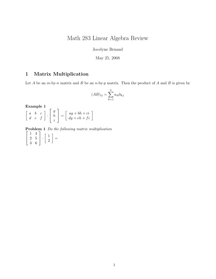
Math 283 Linear Algebra Review Jocelyne Bruand May 25, 2008 1 Matrix Multiplication Let A be an m -by- n matrix and B be an n -by- p matrix. Then the product of A and B is given by n � ( AB ) ij = a ik b kj k =1 Example 1 � a � ag + bh + ci   g � � b c  = h ·  d e f dg + eh + fi i Problem 1 Do the following matrix multiplication � 1  1 4  � 2 5  · =  2 3 6 1

2 Determinant The determinant of a 2-by-2 matrix is given by � � a b � � � = ad − bc � � c d � The determinant of a 3-by-3 matrix is given by � � a b c � � � � = aei + bfg + cdh − afh − bdi − ceg d e f � � � � g h i � � Example 2 � � 1 2 � � � = 1 · 4 − 2 · 3 = − 2 � � 3 4 � In matlab: In R: det([1 2; 3 4]) det(array(c(1,3,2,4), c(2,2))) ans = [1] -2 -2 Problem 2 Calculate the following determinant � � 1 2 3 � � � � 3 2 1 = � � � � 1 2 4 � � 2

3 Matrix Inversion A matrix is invertible if and only if its determinant is non-zero. The inverse matrix A − 1 of the n -by- n matrix A is a unique n -by- n which satisfies AA − 1 = A − 1 A = I n where I n is the n -by- n identity matrix. Example 3 � 1 � 1 � � 2 1 0 2 1 0 ∼ = 3 4 0 1 0 − 2 − 3 1 R 2 ← R 2 − 3 R 1 � 1 � R 1 ← R 1 + R 2 0 − 2 1 ∼ = 3 − 1 R 2 ← − 1 0 1 2 R 2 2 2 In matlab: In R: >> inv([1 2; 3 4]) > solve(array(c(1,3,2,4), c(2,2))) ans = [,1] [,2] -2.0000 1.0000 [1,] -2.0 1.0 1.5000 -0.5000 [2,] 1.5 -0.5   1 2 3 3 2 1 Problem 3 Find the inverse of  .  0 0 1 3

4 Eigenvalues and Eigenvectors The vector � x is an eigenvector for A if there exist a scalar λ such that A� x = λ� x . λ is the eigenvalue corresponding to � x . It can be shown that λ is an eigenvalue of A if and only if det ( A − λI n ) = 0. � 2 � 1 Example 4 We want to find the eigenvalues and eigenvectors of . 0 1 � � 2 − λ 1 � � det ( A − λI n ) = � � 0 1 − λ � � = (2 − λ )(1 − λ ) The roots of (2 − λ )(1 − λ ) are 1 and 2 . These are the eigenvalues of A. Now we want to solve A� x = λ� x . � 2 x 1 + x 2 = λx 1 A� x = λ� x ⇒ x 2 = λx 2 � � c For λ 1 = 1 , x 2 = − x 1 so the eigenvectors have the form . − c � c � For λ 2 = 2 , x 2 = 0 so the eigenvectors have the form . 0 In matlab, In R: >> [V,D] = eig([2 1; 0 1]) > eig = eigen(array(c(2,0,1,1), c(2,2))) V = > eig 1.0000 -0.7071 $values 0 0.7071 [1] 2 1 D = $vectors 2 0 [,1] [,2] 0 1 [1,] 1 -0.7071068 [2,] 0 0.7071068 Note that matlab and R will normalize the eigenvectors.  1 2 3  Problem 4 Find the eigenvalues and eigenvectors of A = 3 2 1  .  0 0 1 4

5

5 Matrix Diagonalization A square matrix A is diagonalizable if there exists an invertible matrix V such that A = V DV − 1 is a diagonal matrix. Matrix diagonalization is the process of finding V and D . One can form D by putting the eigenvalues along the diagonal of a matrix, and V by having the corresponding eigenvectors in each column. Example 5 Let’s look at the previous example. We had λ 1 = 1 and λ 2 = 2 . Therefore, we find � 1 � 0 D = . 0 2 � c � � � c We found the corresponding eigenvectors to be of the forms and respectively, so − c 0 � � 1 1 V = . − 1 0 Now, we can show that � 0 − 1 � V − 1 = 1 1 and � 1 � 0 � 2 � � � � � 1 1 0 − 1 1 V DV − 1 = = = A · · − 1 0 0 2 1 1 0 1   1 2 3 Problem 5 Diagonalize A = 3 2 1  .  0 0 1 Hint: Use previous problem. 6

6 Spectral Decomposition We can obtain the n th power of a matrix by multiplying it with itself n times. So A n = A · A · . . . · A . Now, if A is diagonalizable then we can find V and D such that D = V − 1 AV ⇒ A = V DV − 1 . Thus we can write the following expansion: A n = V DV − 1 · V DV − 1 . . . V DV − 1 = V D n V − 1 . Now, we have V = [ � r 1 � r 2 . . . � r m ] where � r 1 , � r 2 , . . . , � r m are the columns of V so the right eigenvectors  ′  � l 1 ′ are the rows of V − 1 so the tranposes of the . of A . We have V − 1 = ′ , � ′ , . . . , �  where �  .  l 1 l 2 l m .    ′ � l m x = A T � left eigenvectors of A (solution to λ� x ). Then, λ n   0 . . . 0 1 λ n 0 0 . . . V D n V − 1 = V   2  V − 1  . . .  ... . . .   . . .  λ n 0 0 . . . m λ n  0 0   0 0 0  . . . . . . 1 0 0 . . . 0 0 0 . . . 0   V − 1 + . . . + V     V − 1 = V  . . .   . . .  ... ... . . . . . .     . . . . . .   λ n 0 0 . . . 0 0 0 . . . m ′ + � ′ + . . . + � ′ 1 � 2 � m � r 1 λ n r 2 λ n r m λ n = � l 1 l 2 l m ′ + λ n ′ + . . . + λ n ′ . r 1 � r 2 � r m � = λ n 1 � l 1 2 � l 2 m � l m This is the spectral decomposition of A n . Example 6 Let’s continue the previous example. We have � 2 � 1 � 0 � � � � � 1 1 1 0 − 1 V − 1 = A = V = D = . 0 1 − 1 0 0 2 1 1 We can calculate � 2 � 4 � � 2 � 8 � 3 � � 1 3 1 7 A 3 = = = 0 1 0 1 0 1 0 1 If we use the spectral decomposition, we get � 1 � � � � � 1 A 3 = 1 3 + 2 3 � � 0 − 1 1 1 − 1 0 � 1 � 8 − 1 � 8 � = + 0 1 0 0 � 8 7 � = 0 1 7

  1 2 3 Problem 6 Calculate A 3 for A =  using both basic matrix multiplication and spectral 3 2 1  0 0 1 decomposition. 8