Math 211 Math 211 Lecture #6 Mixing Problems January 29, 2001 2 - PowerPoint PPT Presentation
1 Math 211 Math 211 Lecture #6 Mixing Problems January 29, 2001 2 Solving x = a ( t ) x + f ( t ) Solving x = a ( t ) x + f ( t ) Rewrite as x ax = f. Multiply by the integrating factor u ( t ) = e a ( t ) dt .
1 Math 211 Math 211 Lecture #6 Mixing Problems January 29, 2001
2 Solving x ′ = a ( t ) x + f ( t ) Solving x ′ = a ( t ) x + f ( t ) • Rewrite as x ′ − ax = f. • Multiply by the integrating factor u ( t ) = e − � a ( t ) dt . ⋄ Makes the LHS an exact derivative [ ux ] ′ = ux ′ − aux = uf. � • Integrate: u ( t ) x ( t ) = u ( t ) f ( t ) dt + C. • Solve for x ( t ) . Return
3 Mixing Problem 1 Mixing Problem 1 A tank originally holds 500 gallons of pure water. At t = 0 there starts a flow of sugar water into the tank with a concentration of 1 2 lbs/gal at a rate of 5 gal/min. There is also a pipe at the bottom of the tank removing 5 gal/min from the tank. Assume that the sugar is immediately and thoroughly mixed throughout the tank. Find the amount of sugar in the tank after 10 minutes and after 2 hours. Return
4 Model Model • S ( t ) = the amount of sugar in the tank in lbs. • Concentration = pounds per unit volume. ⋄ c ( t ) = S ( t ) lbs gal . V • Modeling is easier in terms of the total amount, S ( t ) . • Draw a picture. Return
5 Balance Law Balance Law • Rate of change = Rate in - Rate out • Rate = volume rate × concentration • For the problem ⋄ Rate in = 5 gal min × 1 gal = 2 . 5 lb lb 2 min ⋄ Rate out = 5 gal lb lb min × S S gal = 500 100 min Return
6 Solution Solution dS dt = Rate in - Rate out = 2 . 5 − S 100 . • General solution: S ( t ) = 250 + Ce − t/ 100 . • Particular solution: S ( t ) = 250(1 − e − t/ 100 ) . Return Balance law
7 Other possible initial conditions Other possible initial conditions • There is initially 20 lbs of sugar in the tank. • The concentration of sugar in the tank at t = 0 is 1 lb/gallon. Solution
8 Mixing Problem 2 Mixing Problem 2 A tank originally holds 500 gallons of sugar water 1 with a concentration of 10 lb/gal. At t = 0 there starts a flow of sugar water into the tank with a concentration of 1 2 lbs/gal at a rate of 5 gal/min. There is also a pipe at the bottom of the tank removing 10 gal/min from the tank. Assume that the sugar is immediately and thoroughly mixed throughout the tank. Find the amount of sugar in the tank after 10 minutes and after 2 hours. Return
9 Solution Solution • Rate in = 5 gal min × 1 gal = 2 . 5 lb lb 2 min • Rate out = 10 gal lb min × S gal V ⋄ V ( t ) = 500 − 5 t. 10 S lb ⋄ Rate out = 500 − 5 t min Balance law Problem Return
10 dS dt = Rate in - Rate out 2 S = 2 . 5 − 100 − t, • General solution: S ( t ) = 2 . 5(100 − t ) + C (100 − t ) 2 . • Particular solution: S ( t ) = 2 . 5(100 − t ) − (100 − t ) 2 . 50
11 Qualitative Analysis Qualitative Analysis • Do solutions always exist? • How many solutions are there? ⋄ To an initial value problem. • Can we predict the behavior of solutions without having a formula? Return
12 Example Example • Initial value problem: sin( t ) y ′ = cos( t ) y +sin 2 ( t ) with y (0) = 1 . • Every solution to the differential equation has the form y ( t ) = t sin t + C sin t. • Hence y (0) = 0 for every solution. The IVP with y (0) = 1 has no solution. Questions Return
13 Existence of Solutions Existence of Solutions • Put the equation sin( t ) y ′ = cos( t ) y + sin 2 ( t ) into normal form y ′ = cos t sin t y + sin t. • The RHS is discontinuous at t = 0 . • If we require the RHS to be continuous there is always a solution to an initial value problem. Example Return
14 Existence Theorem Existence Theorem Suppose the function f ( t, y ) is defined Theorem: and continuous in the rectangle R in the ty -plane. Then given any point ( t 0 , y 0 ) ∈ R , the initial value problem y ′ = f ( t, y ) with y ( t 0 ) = y 0 has a solution y ( t ) defined in an interval containing t 0 . Furthermore the solution will be defined at least until the solution curve t → ( t, y ( t )) leaves the rectangle R. Example Return
15 What is a Theorem? What is a Theorem? • A theorem is a logical statement. • It contains ⋄ hypotheses (the assumptions made) ⋄ and conclusions • The conclusions are guaranteed to be true if the hypotheses are true. Return
16 Example of a “Theorem” Example of a “Theorem” If it rains the sidewalks get wet. • Hypothesis — If it rains • Conclusion — the sidewalks get wet Existence theorem Theorem
17 Mathematics and Proof Mathematics and Proof • Theorems are proved by logical deduction. • All of mathematics comes from a small number of very basic assumptions. ⋄ Called axioms or postulates . • True of all parts of mathematics. ⋄ An algebraic derivation is an example of a proof. • Definitions are not theorems. Existence theorem
18 Interval of Existence Interval of Existence • Example: y ′ = 1 + y 2 with y (0) = 0 . • RHS f ( t, y ) = 1 + y 2 is defined and continuous on the whole ty -plane. The rectangle R can be any rectangle in the plane. • Solution y ( t ) = tan t “blows up” at t = ± π/ 2 . • Thus the size of the rectangle on which f ( t, y ) is continuous does not say much about the interval of existence. Existence theorem Return
19 Uniqueness of Solutions Uniqueness of Solutions • How many solutions does an initial value problem have? • The uniqueness of solutions to an initial value problem is the mathematical equivalent of being able to predict results in science and engineering. • We will need slightly stronger restrictions to ensure uniqueness than we needed for existence. Questions
20 Uniqueness of Solutions Uniqueness of Solutions • Initial value problem y ′ = y 1 / 3 with y (0) = 0 . • The constant function y 1 ( t ) = 0 is a solution. • Solve by separation of variables to find that � 3 / 2 � 2 t , if t > 0 3 y 2 ( t ) = 0 , if t ≤ 0 . is also a solution. Return Existence theorem
21 Suppose f ( t, y ) , ∂f/∂y are continuous Theorem: in the rectangle R . Let � � ∂f � � M = max ∂y ( t, y ) � . � � ( t,y ) ∈ R � Suppose that ( t 0 , x 0 ) and ( t 0 , y 0 ) both lie in R , and x ′ = f ( t, x ) , x ( t 0 ) = x 0 & y ′ = f ( t, y ) , y ( t 0 ) = y 0 . Then as long as ( t, x ( t )) and ( t, y ( t )) stay in R we have | x ( t ) − y ( t ) | ≤ | x 0 − y 0 | e M | t − t 0 | . Existence theorem Return
22 Uniqueness Theorem Uniqueness Theorem Suppose the function f ( t, y ) and its partial Theorem: derivative ∂f/∂y are continuous in the rectangle R in the ty -plane. Suppose that ( t 0 , x 0 ) ∈ R . Suppose that x ′ = f ( t, x ) y ′ = f ( t, y ) , and and that x ( t 0 ) = y ( t 0 ) = x 0 . Then as long as ( t, x ( t )) and ( t, y ( t )) stay in R we have x ( t ) = y ( t ) . Return Example Inequality
23 Geometric Interpretation Geometric Interpretation • Solution curves cannot cross. • They cannot even touch at one point. • y ′ = ( y − 1)(cos t − y ) and y (0) = 2 . Show y ( t ) > 1 for all t. • y ′ = y − (1 − t ) 2 and y (0) = 0 . Show that y ( t ) < 1 + t 2 for all t. Unigueness theorem
24 E & U for Linear Equations E & U for Linear Equations Suppose that a ( t ) and g ( t ) are Theorem: continuous on an interval I = ( a, b ) . Then given t 0 ∈ I and any y 0 , the initial value problem y ′ = a ( t ) y + g ( t ) with y ( t 0 ) = y 0 has a unique solution y ( t ) which exists for all t ∈ I. • Notice that the RHS is ∂f f ( t, y ) = a ( t ) y + g ( t ) , and ∂y = a ( t ) . These are continuous for t ∈ I and all y . Existence theorem Uniqueness theorem
25 DFIELD5 DFIELD5 Get a geometric look at existence and uniqueness.
Recommend
More recommend
Explore More Topics
Stay informed with curated content and fresh updates.
