Math 211 Math 211 Lecture #29 Phase Plane Portraits Systems of - PowerPoint PPT Presentation
1 Math 211 Math 211 Lecture #29 Phase Plane Portraits Systems of Higher Dimension November 4, 2002 2 Planar System x = A x Planar System x = A x Equilibrium points for the system Set of equilibrium points equals null( A ) .
1 Math 211 Math 211 Lecture #29 Phase Plane Portraits Systems of Higher Dimension November 4, 2002
2 Planar System x ′ = A x Planar System x ′ = A x • Equilibrium points for the system � Set of equilibrium points equals null( A ) . � A nonsingular ⇒ only equilibrium point is 0 . • Can we list the types of all possible equilibrium points for planar linear systems? � We will do the six most important cases. � Look at solution curves in the phase plane. Return
3 Distinct Real Eigenvalues Distinct Real Eigenvalues • p ( λ ) = λ 2 − Tλ + D with T 2 − 4 D > 0 . √ √ T 2 − 4 D T 2 − 4 D λ 1 = T − < λ 2 = T + 2 2 • Eigenvectors v 1 and v 2 . General solution x ( t ) = C 1 e λ 1 t v 1 + C 2 e λ 2 t v 2 • λ 1 < 0 < λ 2 Saddle point. • λ 1 < λ 2 < 0 Nodal sink. • 0 < λ 1 < λ 2 Nodal source. Return Plan
4 Complex Eigenvalues Complex Eigenvalues • p ( λ ) = λ 2 − Tλ + D with T 2 − 4 D < 0 λ = α + iβ λ = α − iβ. and • Eigenvector w = v 1 + i v 2 associated to λ . • General solution x ( t ) = C 1 e αt [cos βt · v 1 − sin βt · v 2 ] + C 2 e αt [sin βt · v 1 + cos βt · v 2 ] • α = Re( λ ) = 0 Center. • α = Re( λ ) < 0 Spiral sink. • α = Re( λ ) > 0 Spiral source. Return
5 Planar Systems Planar Systems � a 11 a 12 � A = a 21 a 22 • The characteristic polynomial is p ( λ ) = λ 2 − Tλ + D . where � T = tr A = a 11 + a 22 and � D = det A = a 11 a 22 − a 12 a 21 . • The eigenvalues are √ T 2 − 4 D λ 1 , λ 2 = T ± . 2 Return
6 • λ 1 & λ 2 are the roots of p ( λ ) = λ 2 − Tλ + D , so p ( λ ) = ( λ − λ 1 )( λ − λ 2 ) = λ 2 − ( λ 1 + λ 2 ) λ + λ 1 λ 2 • Hence, T = λ 1 + λ 2 and D = λ 1 λ 2 . • Duality between ( λ 1 , λ 2 ) and ( T, D ) . • We will represent a system by the location of ( T, D ) in the TD -plane — the trace-determinant plane. Return
7 Trace-Determinant Plane Trace-Determinant Plane • T 2 − 4 D > 0 � ⇒ distinct real eigenvalues λ 1 & λ 2 � D = λ 1 λ 2 < 0 ⇒ Saddle point. � D = λ 1 λ 2 > 0 ⇒ Eigenvalues have the same sign. ◮ T = λ 1 + λ 2 > 0 ⇒ Nodal source. ◮ T = λ 1 + λ 2 < 0 ⇒ Nodal sink. Return Duality
8 • T 2 − 4 D < 0 ⇒ complex eigenvalues λ = α + iβ λ = α − iβ. and � T = λ + λ = 2 α > 0 ⇒ Spiral source. � T = λ + λ = 2 α < 0 ⇒ Spiral sink. � T = λ + λ = 2 α = 0 ⇒ Center. Return Duality TD plane
9 Types of Equilibrium Points Types of Equilibrium Points • Generic types � Saddle, nodal source, nodal sink, spiral source, and spiral sink. � All occupy large open subsets of the trace-determinant plane. • Nongeneric types � Center and many others. Occupy pieces of the boundaries between the generic types. Return
10 Higher Dimensional Systems Higher Dimensional Systems x ′ = A x • A is a real n × n matrix. • If λ is an eigenvalue and v � = 0 is an associated eigenvector, then x ( t ) = e λt v is a solution. • Much like the planar case, but now we need n linearly independent solutions. • We no longer have the easy way to compute the characteristic polynomial p ( λ ) = det( A − λI ) . Return
11 Suppose that λ 1 , . . . , λ k are distinct Proposition: eigenvalues of A , and that v 1 , . . . , v k are associated nonzero eigenvectors. Then v 1 , . . . , v k are linearly independent. Suppose the n × n real matrix A has n Theorem: distinct eigenvalues λ 1 , . . . , λ n , and that v 1 , . . . , v n are associated nonzero eigenvectors. Then the exponential solutions x i ( t ) = e λ i t v i , 1 ≤ i ≤ n form a fundamental set of solutions for the system x ′ = A x . Return
12 Examples: Examples: − 2 3 − 4 • A = 0 1 0 0 4 − 1 17 − 30 − 8 • A = 16 − 29 − 8 − 12 24 7 � Use M ATLAB . Return
13 Complex Eigenvalues Complex Eigenvalues A a real n × n matrix with a complex eigenvalue λ and associate eigenvector w . • ⇒ λ is an eigenvalue and w is an associated nonzero eigenvector. • Complex valued solutions: z ( t ) = e λt w z ( t ) = e λt w . • Real solutions: x ( t ) = Re( z ( t )) y ( t ) = Im( z ( t )) . Return
14 Example Example 21 10 4 A = − 70 − 31 − 10 30 10 − 1 • The theorem applies if some of the eigenvalues are complex and we replace complex conjugate pairs of solutions by their real and imaginary parts. Return
15 Repeated Eigenvalues – Example 1 Repeated Eigenvalues – Example 1 − 5 − 10 6 A = 8 19 − 12 12 30 − 19 • p ( λ ) = ( λ + 3)( λ + 1) 2 • λ 1 = − 3 � Eigenspace has dimension 1 ⇒ one exponential solution x 1 ( t ) = e − 3 t ( − 1 / 3 , 2 / 3 , 1) T Return Example 1a Example 2 Example 2a Analysis
16 • λ 2 = − 1 � Eigenspace has dimension 2 ⇒ two linearly independent exponential solutions � Eigenspace has basis v 2 = ( − 5 / 2 , 1 , 0) T and v 3 = (3 / 2 , 0 , 1) T . � Linearly independent solutions − 5 / 2 3 / 2 x 2 ( t ) = e − t x 3 ( t ) = e − t 1 0 & 0 1 • x 1 , x 2 , and x 3 are a fundamental set of solutions. Return Example 1 Example 2 Example 2a Analysis
17 Repeated Eigenvalues – Example 2 Repeated Eigenvalues – Example 2 1 2 − 1 A = − 4 − 7 4 − 4 − 4 1 • p ( λ ) = ( λ + 3)( λ + 1) 2 • λ 1 = − 3 � Eigenspace has dimension 1 ⇒ one exponential solution x 1 ( t ) = e − 3 t ( − 1 / 2 , 3 / 2 , 1) T Return Example 1 Example 1a Example 2a Analysis
18 • λ 2 = − 1 � Eigenspace has dimension 1 ⇒ only one exponential solution − 1 / 2 x 2 ( t ) = e − t 1 1 • Need a third solution. • Need a new idea. Return Example 1 Example 1a Example 2 Analysis
19 Multiplicities Multiplicities A an n × n matrix • Distinct eigenvalues λ 1 , . . . , λ k . • The characteristic polynomial is p ( λ ) = ( λ − λ 1 ) q 1 ( λ − λ 2 ) q 2 · . . . · ( λ − λ k ) q k . • The algebraic multiplicity of λ j is q j . • The geometric multiplicity of λ j is d j , the dimension of the eigenspace of λ j . Return Example 1 Example 1a Example 2 Example 2a
20 • We always have: � q 1 + q 2 + · · · + q k = n . � 1 ≤ d j ≤ q j . � There are d j linearly independent exponential solutions corresponding to λ j . � If d j = q j for all j we have n linearly independent solutions. • If d j < q j we have trouble. Return Example 1 Example 1a Example 2 Example 2a
Recommend
More recommend
Explore More Topics
Stay informed with curated content and fresh updates.
