Mata Programming I Christopher F Baum Boston College and DIW Berlin - PowerPoint PPT Presentation
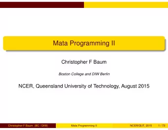
Mata Programming I Christopher F Baum Boston College and DIW Berlin NCER, Queensland University of Technology, August 2015 Christopher F Baum (BC / DIW) Mata Programming I NCER/QUT, 2015 1 / 73 Introduction to Mata Introduction to Mata We
Mata Programming I Christopher F Baum Boston College and DIW Berlin NCER, Queensland University of Technology, August 2015 Christopher F Baum (BC / DIW) Mata Programming I NCER/QUT, 2015 1 / 73
Introduction to Mata Introduction to Mata We now turn to a second way in which you may use Stata programming techniques: by taking advantage of Mata. Since the release of version 9, Stata has contained a full-fledged matrix programming language, Mata, with most of the capabilities of MATLAB , R , Ox or Gauss. You can use Mata interactively, or you can develop Mata functions to be called from Stata. Christopher F Baum (BC / DIW) Mata Programming I NCER/QUT, 2015 2 / 73
Introduction to Mata Mata functions may be particularly useful where the algorithm you wish to implement already exists in matrix-language form. It is quite straightforward to translate the logic of other matrix languages into Mata: much more so than converting it into Stata’s matrix language. A large library of mathematical and matrix functions is provided in Mata, including optimization routines, equation solvers, decompositions, eigensystem routines and probability density functions. Mata functions can access Stata’s variables and can work with virtual matrices ( views ) of a subset of the data in memory. Mata also supports file input/output. Christopher F Baum (BC / DIW) Mata Programming I NCER/QUT, 2015 3 / 73
Introduction to Mata Circumventing the limits of Stata’s matrix language Circumventing the limits of Stata’s matrix language Mata circumvents the limitations of Stata’s traditional matrix commands. Stata matrices must obey the maximum matsize: 800 rows or columns in Stata/IC. Thus, code relying on Stata matrices is fragile. Stata’s matrix language does contain commands such as matrix accum which can build a cross-product matrix from variables of any length, but for many applications the limitation of matsize is binding. Christopher F Baum (BC / DIW) Mata Programming I NCER/QUT, 2015 4 / 73
Introduction to Mata Circumventing the limits of Stata’s matrix language Even in Stata/SE or Stata/MP , with the possibility of a much larger matsize , Stata’s matrices have another drawback. Large matrices consume large amounts of memory, and an operation that converts Stata variables into a matrix or vice versa will require at least twice the memory needed for that set of variables. Christopher F Baum (BC / DIW) Mata Programming I NCER/QUT, 2015 5 / 73
Introduction to Mata Circumventing the limits of Stata’s matrix language The Mata programming language can sidestep these memory issues by creating matrices with contents that refer directly to Stata variables—no matter how many variables and observations may be referenced. These virtual matrices, or views , have minimal overhead in terms of memory consumption, regardless of their size. Unlike some matrix programming languages, Mata matrices can contain either numeric elements or string elements (but not both). This implies that you can use Mata productively in a list processing environment as well as in a numeric context. For example, a prominent list-handling command, Bill Gould’s adoupdate , is written almost entirely in Mata. viewsource adoupdate.ado reveals that only 22 lines of code (out of 1,193 lines) are in the ado-file language. The rest is Mata. Christopher F Baum (BC / DIW) Mata Programming I NCER/QUT, 2015 6 / 73
Introduction to Mata Speed advantages Speed advantages Last but by no means least, ado-file code written in the matrix language with explicit subscript references is slow . Even if such a routine avoids explicit subscripting, its performance may be unacceptable. For instance, David Roodman’s xtabond2 can run in version 7 or 8 without Mata, or in version 9 onwards with Mata. The non-Mata version is an order of magnitude slower when applied to reasonably sized estimation problems. Christopher F Baum (BC / DIW) Mata Programming I NCER/QUT, 2015 7 / 73
Introduction to Mata Speed advantages In contrast, Mata code is automatically compiled into bytecode , like Java, and can be stored in object form or included in-line in a Stata do-file or ado-file. Mata code runs many times faster than the interpreted ado-file language, providing significant speed enhancements to many computationally burdensome tasks. Christopher F Baum (BC / DIW) Mata Programming I NCER/QUT, 2015 8 / 73
Introduction to Mata An efficient division of labor An efficient division of labor Mata interfaced with Stata provides for an efficient division of labor. In a pure matrix programming language, you must handle all of the housekeeping details involved with data organization, transformation and selection. In contrast, if you write an ado-file that calls one or more Mata functions, the ado-file will handle those housekeeping details with the convenience features of the syntax and marksample statements of the regular ado-file language. When the housekeeping chores are completed, the resulting variables can be passed on to Mata for processing. Results produced by Mata may then be accessed by Stata and formatted with commands like estimates display . Christopher F Baum (BC / DIW) Mata Programming I NCER/QUT, 2015 9 / 73
Introduction to Mata An efficient division of labor Mata can access Stata variables, local and global macros, scalars and matrices, and modify the contents of those objects as needed. If Mata’s view matrices are used, alterations to the matrix within Mata modifies the Stata variables that comprise the view. Christopher F Baum (BC / DIW) Mata Programming I NCER/QUT, 2015 10 / 73
Mata language elements Operators Language syntax: Operators To understand Mata syntax, you must be familiar with its operators. The comma is the column-join operator, so : r1 = ( 1, 2, 3 ) creates a three-element row vector. We could also construct this vector using the row range operator (..) as : r1 = (1..3) The backslash is the row-join operator, so c1 = ( 4 5 6 ) creates a three-element column vector. We could also construct this vector using the column range operator (::) as : c1 = (4::6) Christopher F Baum (BC / DIW) Mata Programming I NCER/QUT, 2015 11 / 73
Mata language elements Operators We may combine the column-join and row-join operators: m1 = ( 1, 2, 3 \ 4, 5, 6 \ 7, 8, 9 ) creates a 3 × 3 matrix. The matrix could also be constructed with the row range operator: m1 = ( 1..3 \ 4..6 \ 7..9 ) Christopher F Baum (BC / DIW) Mata Programming I NCER/QUT, 2015 12 / 73
Mata language elements Operators The prime (or apostrophe) is the transpose operator, so r2 = ( 1 \ 2 \ 3 ) ´ is a row vector. The comma and backslash operators can be used on vectors and matrices as well as scalars, so r3 = r1, c1 ´ will produce a six-element row vector, and c2 = r1 ´ \ c1 creates a six-element column vector. Matrix elements can be real or complex, so 2 - 3 i refers to a √ complex number 2 − 3 × − 1. Christopher F Baum (BC / DIW) Mata Programming I NCER/QUT, 2015 13 / 73
Mata language elements Operators The standard algebraic operators plus ( + ), minus ( − ) and multiply ( ∗ ) work on scalars or matrices: g = r1 ´ + c1 h = r1 * c1 j = c1 * r1 In this example h will be the 1 × 1 dot product of vectors r1, c1 while j is their 3 × 3 outer product. Christopher F Baum (BC / DIW) Mata Programming I NCER/QUT, 2015 14 / 73
Mata language elements Element-wise calculations and the colon operator Element-wise calculations and the colon operator One of Mata’s most powerful features is the colon operator . Mata’s algebraic operators, including the forward slash ( / ) for division, also can be used in element-by-element computations when preceded by a colon: k = r1 ´ :* c1 will produce a three-element column vector, with elements as the product of the respective elements: k i = r 1 i c 1 i , i = 1 , . . . , 3. Christopher F Baum (BC / DIW) Mata Programming I NCER/QUT, 2015 15 / 73
Mata language elements Element-wise calculations and the colon operator Mata’s colon operator is very powerful, in that it will work on nonconformable objects, or what Mata considers c-conformable objects. These include cases where two objects have the same number of rows (or the same number of columns), but one is a matrix and the other is a vector or scalar. For example: r4 = ( 1, 2, 3 ) m2 = ( 1, 2, 3 \ 4, 5, 6 \ 7, 8, 9 ) m3 = r4 :+ m2 m4 = m1 :/ r1 adds the row vector r4 to each row of the 3 × 3 matrix m2 to form m3 , and divides the elements of each row of matrix m1 by the corresponding elements of row vector r1 to form m4 . Mata’s scalar functions will also operate on elements of matrices: d = sqrt(c) will take the element-by-element square root, returning missing values where appropriate. Christopher F Baum (BC / DIW) Mata Programming I NCER/QUT, 2015 16 / 73
Recommend
More recommend
Explore More Topics
Stay informed with curated content and fresh updates.
