MATA IMPLEMENTATION OF GAUSS-LEGENDRE QUADRATURE IN THE M-ESTIMATION - - PowerPoint PPT Presentation

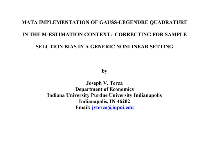
MATA IMPLEMENTATION OF GAUSS-LEGENDRE QUADRATURE IN THE M-ESTIMATION CONTEXT: CORRECTING FOR SAMPLE SELCTION BIAS IN A GENERIC NONLINEAR SETTING by Joseph V. Terza Department of Economics Indiana University Purdue University Indianapolis Indianapolis, IN 46202 Email: jvterza@iupui.edu

M-Estimation and Integration

• - We focus on cases in which the objective function for the relevant M-Estimator

involves non-closed-form integration.

• - Prominent cases include:
• - Nonlinear models with endogenous treatments
• - Nonlinear models with sample selection
• - Nonlinear panel data models with random effects
• - Count data models with unobserved heterogeneity for accommodating

non-equi-dispersed data.

• - Etc.

2

Modeling Sample Selection in the Fully Parametric Case

• - Some definitions (see Terza, 2009)
• - Y ≡ the observable version of the outcome of interest
• X ≡ the vector of observable regressors
• u

X ≡ the scalar comprising the unobservable regressors

• u

[X X ]  X

• - Suppose that the relevant underlying potential outcomes specification satisfies the

requisite conditions establishing the legitimacy of following data generating process (DGP) specification (see Terza, 2019)

• u

(Y | )

• u

pmf / pdf(Y | ) pmf / pdf(Y | X , X ) f (Y, X , X ; γ)  

X

X

(1) where (Y |

)

f ( . )

X

is a known function and γ is a vector of unknown parameters.

Terza, J.V. (2009): “Parametric Nonlinear Regression with Endogenous Switching,” Econometric Reviews, 28, 555-580. Terza, J.V. (2019): “Regression-Based Causal Analysis from the Potential Outcomes Perspective,” Journal of Econometric Methods, published online ahead of print, DOI: https://doi.org/10.1515/jem-2018-0030.

3

Modeling Sample Selection in the Fully Parametric Case (cont’d)

• - In addition the DGP includes a “selection rule”

u

S I(C(W,X ,δ))  (2) where S ≡ an observable binary variable

• W

[X W ]



 W is a vector of variables not included in

• X

δ is a vector of unknown parameters C( . ) represents a “criterion” to be satisfied by W,

u

X and δ. The selection rule maintains that Y is observable only if S

1  .

4

Sample Selection Bias

• - Ignoring the presence of

u

X in (1) and (2) while implementing an M-estimator (in this case a maximum likelihood estimator [MLE]) based solely on (1) with

u

X suppressed will likely result in a kind of omitted variable bias in the estimate of γ.

5

Correcting for Sample Selection Bias in M-Estimation

• - Continuing with our fully parametric example, let us maintain the following

specific form for the selection rule

u

S I(Wδ X 0)    . (3)

• - Let us also suppose that the distribution of (

u

X | W) is known with pdf

u

(X |W) u

g (X , W) and cdf

u

(X |W) u

G (X , W), respectively.

• - Under these conditions, Terza (2009) shows that

(Y,S|W)

pdf(Y, S | W) f (Y,S,W; γ, δ) 

u u

S 1 S (Y | )

• u

(X |W) u u (X |W) Wδ

f (Y, X , X ; γ) g (X , W)dX G ( Wδ)

  

         

X

. (4)

6

Correcting for Sample Selection Bias in M-Estimation (cont’d)

• - Using (4) we can construct the following log-likelihood function

i (Y,S|W) i i i

q(γ, δ, Z ) ln[f (Y ,S ,W ; γ, δ)]      . (5) where

i i i i

[ Z Y W S ]  is the data vector.

• - The following M-estimator (MLE) is consistent for [γ

δ] is the following

n i i 1 [γ δ]

argmax q(γ, δ, Z )





 

  . (6)

7

Correcting for Sample Selection Bias in M-Estimation (cont’d)

• - The problem with this approach is that

i

q(γ, δ, Z )   involves a typically non-closed- form integral, viz.

u i

(Y | ) i io u (X |W) u i u W δ

f (Y , X , X ; γ) g (X , W )dX

   X

(7) that must be calculated for each observation in the sample at each iteration of the

• ptimization algorithm for (6).

8

A Bit of Mata Code to Solve this Problem

• - I have written a Mata function that implements Gauss-Legendre quadrature for

approximating non-closed-form integrals like the one in (7).

• - This function is called “quadleg” and is implemented in the following way:

integralvec=quadleg(&integrand(),limits,wtsandabs) where integrand specifies the name of a Mata function for the relevant integrand (should be coded so as to accommodate n×R matrix arguments – where n is the number of observations and R is the number of abscissae and weights to be used for the quadrature). limits is an n×2 matrix of integration limits (observation-specific) – first and second columns contain lower and upper limits of integration, respectively.

9

A Bit of Mata Code to Solve this Problem (cont’d) wtsandabs R×2 matrix of weights and abscissae to be used for the quadrature integralvec function output -- n×1 vector of integral values. Prior to invoking quadleg, the requisite Gauss-Legendre quadrature weights and abscissae must be obtained using the function “GLQwtsandabs” which is called in the following way wtsandabs = GLQwtsandabs(quadpts) where quadpts is the number of weights and abscissae to be used for the quadrature.

10

Application to Sample Selection Modeling and Estimation

• - Recall the classical sample selection model in which

Y ≡ the wage offer (not the observed wage)

• u

[X X ]  X ≡ wage offer determinants

u

S I(Wδ X 0)    = 1 if employed, 0 if not W ≡ employment determinants

• - For this illustration, we assume that

u

(X | W) is standard normally distributed.

• - We consider three specifications for the distribution of (Y |

) X [which, of course defines (Y |

)

• u

f (Y, X , X ; γ)

X

]: I) Normal with mean β X and variance

2

σ ; II) Log-

Normal with log mean β X and log variance

2

σ ; and III) Generalized Gamma (GG)

with parameters β X ,

2

σ and κ.

11

Application to Sample Selection Modeling and Estimation (cont’d)

• - Neither Case I nor Case II is problematic as both of these cases can be estimated

in Stata using the packaged “heckman” command.

• - We therefore focus on Case III in which (Y |

) X is GG distributed and

(Y | )

• u

f (Y, X , X ; γ)

X

is the GG pdf with

2

γ = [β σ κ]  [for the explicit formulation

• f the GG pdf and its properties see Manning, Mullahy and Basu (2005)].
• - In this case the problematic integral is

2 u u Wδ

gg(Y; β, σ , κ) φ(X )dX

  

X (8) where

2

gg(Y; β, σ , κ) X denotes the GG pdf appropriately parameterized.

Manning, W.G, Basu, A. and Mullahy, L. (2005): “Generalized Modeling Approaches to Risk Adjustment of Skewed Outcomes Data,” Journal of Health Economics, 24, 465-488.

12

Application to Sample Selection Modeling and Estimation (cont’d)

• - We begin by noting that the codes for the quadleg and GLQwtsandabs

functions should be inserted in your Mata program and should remain unaltered.

• - Recall that the quadleg function has three arguments:

1) The integrand function. In our case this is

2 u

gg(Y; β, σ , κ) φ(X ) X

13

Application to Sample Selection Modeling and Estimation (cont’d) The code for this is

/************************************************* ** Mata Function to compute the integrand for ** objective function (log-liklihood) ** to be used by the Mata moptimize procedure. *************************************************/ real matrix modelintegrand(xxu){ /************************************************* ** Set necessary externals. *************************************************/ external y external xb external bu external lnsigma external kappa /************************************************* ** GG reparameterization (see Manning et al., 2005). *************************************************/ mmu=xb:+xxu:*bu ggamm=1:/(abs(kappa):^2) z=sign(kappa):*(ln(y):-mmu):/exp(lnsigma) u = ggamm:*exp(abs(kappa):*z)

14

Application to Sample Selection Modeling and Estimation (cont’d) The code continued...

/************************************************* ** Vector of GG pdf values. *************************************************/ GGprob=(ggamm:^ggamm):*exp(z:*sqrt(ggamm):-u)/* */:/(exp(lnsigma):*y:*sqrt(ggamm):*gamma(ggamm)) /************************************************* ** Vector of integrand values. *************************************************/ integrandvals=GGprob:*normalden(xxu) /************************************************* ** Return result. *************************************************/ return(integrandvals) }

15

Application to Sample Selection Modeling and Estimation (cont’d) 2) An n×2 matrix of integration limits (observation-specific) for (8)– first and second columns contain lower and upper limits of integration, respectively. The code for this is

/************************************************* ** Construct the obs x 2 matrix of ** observation-specific integration limits. *************************************************/ limita= -vd limitb= 8:*J(rows(vd),1,1) limits=limita,limitb

which is placed in the code for the moptimize objective function – the function that calls quadleg.

16

Application to Sample Selection Modeling and Estimation (cont’d) 3) The R×2 matrix of Gauss-Legendre weights and abscissae The code for this is

/************************************************* ** Compute the matrix of quadrature wts and ** abcissae. *************************************************/ wtsandabs=GLQwtsandabs(quadpts)

17

Running the Code on Data

• - We applied all three models

Case I) Normal with mean β X and variance

2

σ [Stata heckman command]

Case II) Log-Normal with log mean β X and log variance

2

σ [Stata heckman]

Case III) Generalized Gamma (GG) with parameters β X ,

2

σ and κ [Mata with

moptimize and quadleg]. To the wage offer data analyzed by Fishback and Terza (1987).

• - As a summary estimator we used the average treatment effect (ATE) of disability

(a binary variable) on wage offers.

Fishback, P. and Terza, J. (1989). "Are Estimates of Sex Discrimination by Employers Robust? The Use of Never- Marrieds," Economic Inquiry, 27, 271-285.

18

Results Model ATE t-Stat % Difference v. GG Normal

• 1.47
• 4.33

13% Log-Normal

• 1.87
• 9.49

11% Generalized Gamma

• 1.69
• 8.56

Wald test of GG vs. Log-Normal (Ho: κ  0) Wald Stat = 3.34 Asymptotic standard t-stats for Log-Normal and GG ATE estimates obtained using Terza (2016, 2017).

Terza, J.V. (2016): “Inference Using Sample Means of Parametric Nonlinear Data Transformations,” Health Services Research, 51, 1109-1113. Terza, J.V. (2017): “Causal Effect Estimation and Inference Using Stata,” the Stata Journal, 939-961.