Marginalization Simplest multivariate problem: X = ( X 1 , . . . , X - PDF document

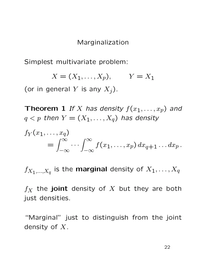
Marginalization Simplest multivariate problem: X = ( X 1 , . . . , X p ) , Y = X 1 (or in general Y is any X j ). Theorem 1 If X has density f ( x 1 , . . . , x p ) and q < p then Y = ( X 1 , . . . , X q ) has density f Y ( x 1 , . . . , x q ) � ∞ � ∞ = −∞ f ( x 1 , . . . , x p ) dx q +1 . . . dx p . −∞ · · · f X 1 ,...,X q is the marginal density of X 1 , . . . , X q f X the joint density of X but they are both just densities. “Marginal” just to distinguish from the joint density of X . 22

Example : The function f ( x 1 , x 2 ) = Kx 1 x 2 1( x 1 > 0 , x 2 > 0 , x 1 + x 2 < 1) is a density provided � ∞ � ∞ P ( X ∈ R 2 ) = −∞ f ( x 1 , x 2 ) dx 1 dx 2 = 1 . −∞ The integral is � 1 � 1 − x 1 K x 1 x 2 dx 1 dx 2 0 0 � 1 0 x 1 (1 − x 1 ) 2 dx 1 / 2 = K = K (1 / 2 − 2 / 3 + 1 / 4) / 2 = K/ 24 so K = 24. The marginal density of x 1 is � ∞ f X 1 ( x 1 ) = −∞ 24 x 1 x 2 × 1( x 1 > 0 , x 2 > 0 , x 1 + x 2 < 1) dx 2 � 1 − x 1 =24 x 1 x 2 1(0 < x 1 < 1) dx 2 0 =12 x 1 (1 − x 1 ) 2 1(0 < x 1 < 1) . This is a Beta(2 , 3) density. 23

General problem has Y = ( Y 1 , . . . , Y q ) with Y i = g i ( X 1 , . . . , X p ). Case 1 : q > p . • Y won’t have density for “smooth” g . • Y will have a singular or discrete distribu- tion. • Problem rarely of real interest. • (But, e.g., residuals have singular distribu- tion.) 24

Case 2 : q = p . • We use a change of variables formula • Generalizes the one derived above for the case p = q = 1. 25

Case 3 : q < p . • Pad out Y –add on p − q more variables (carefully chosen) • say Y q +1 , . . . , Y p . • Find functions g q +1 , . . . , g p . • Define for q < i ≤ p , Y i = g i ( X 1 , . . . , X p ) and Z = ( Y 1 , . . . , Y p ) . • Choose g i so that we can use change of variables on g = ( g 1 , . . . , g p ) to compute f Z . • Find f Y by integration: f Y ( y 1 , . . . , y q ) = � ∞ � ∞ −∞ · · · −∞ f Z ( y 1 , . . . , y q , z q +1 , . . . , z p ) dz q +1 . . . dz p 26

Change of Variables: general Suppose Y = g ( X ) ∈ R p with X ∈ R p having density f X . Assume g is a one to one (“injective”) map, i.e., g ( x 1 ) = g ( x 2 ) if and only if x 1 = x 2 . Find f Y : Step 1: Solve for x in terms of y : x = g − 1 ( y ). Step 2: Use basic equation: f Y ( y ) dy = f X ( x ) dx and rewrite it in the form f Y ( y ) = f X ( g − 1 ( y )) dx dy . Interpretation of derivative dx dy when p > 1: � �� � dx ∂x i � � dy = � det � � � � ∂y j � which is the so called Jacobian . 27

Equivalent formula inverts the matrix: f Y ( y ) = f X ( g − 1 ( y )) � dy � � � � dx � This notation means � ∂y 1 ∂y 1 ∂y 1 �   · · · � � ∂x 1 ∂x 2 ∂x p � � dy � � . �   � . � � . � = det �   � � � dx �   � � ∂y p ∂y p ∂y p � �   · · · � � ∂x 1 ∂x 2 ∂x p � � but with x replaced by the corresponding value of y , that is, replace x by g − 1 ( y ). 28

Example : The density − x 2 1 + x 2 � � f X ( x 1 , x 2 ) = 1 2 2 π exp 2 is the standard bivariate normal density . Let Y = ( Y 1 , Y 2 ) where � X 2 1 + X 2 Y 1 = 2 and 0 ≤ Y 2 < 2 π is angle from the positive x axis to the ray from the origin to the point ( X 1 , X 2 ). I.e., Y is X in polar co-ordinates. Problem is to find joint density of Y 1 and Y 2 . 29

Step 1 : Solve for x in terms of y : = Y 1 cos( Y 2 ) X 1 = Y 1 sin( Y 2 ) X 2 Thus g ( x 1 , x 2 ) = ( g 1 ( x 1 , x 2 ) , g 2 ( x 1 , x 2 )) � x 2 1 + x 2 = ( 2 , argument( x 1 , x 2 )) g − 1 ( y 1 , y 2 ) ( g − 1 1 ( y 1 , y 2 ) , g − 1 = 2 ( y 1 , y 2 )) = ( y 1 cos( y 2 ) , y 1 sin( y 2 )) � � � �� � dx cos( y 2 ) − y 1 sin( y 2 ) � � � � = � det � � � � sin( y 2 ) y 1 cos( y 2 ) � dy � � � � � � = y 1 . 30